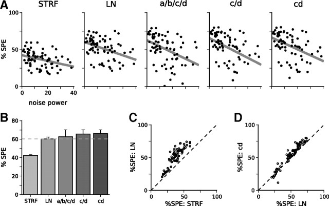
Figure 3.

Including SCKs in models of neural responses improves their predictive power over the LN model; this is further improved by simplifying the model. A, Model predictive power, as measured by Sahani and Linden (2003). Model names are defined in Materials and Methods. For each model, scatter plots show the cross-validated prediction scores across all 77 units. These are calculated as the percentage of the signal power (%SPE) of the unit captured by the model on the prediction dataset and shown as a function of the normalized noise power in the responses of the unit. Gray line shows the extrapolation of prediction scores to an idealized zero-noise unit, producing a lower bound on the overall predictive power of the model over the population of auditory cortical units. The upper bound on predictive power has been omitted for clarity. B, Summary of predictive powers for the models in A. Solid bars show the lower bound (as plotted in A) from cross-validation; error bars show the upper bound from the training dataset. Although adding a full set of contrast kernels (a/b/c/d) leads to a modest improvement in prediction scores over the LN model, the large number of parameters in the full model leads to overfitting. Rendering a and b contrast independent reduces overfitting and improves prediction scores (the c/d model). The best-performing model is the cd model, with a shared contrast kernel between c and d. C, Comparison between prediction scores for the LN model and for the STRF model, on a unit-by-unit basis. D, Comparison between the LN model and cd model on a unit-by-unit basis.