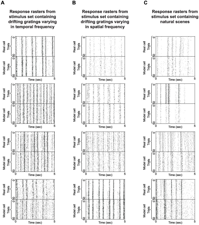
Figure 8. Response rasters for the first 12 cells shown in Fig. 4.

Fig. 4 shows real and model cell performance using three sets of stimuli. Here we show rasters of the underlying responses. A. Rasters for the responses to the drifting gratings that varied in temporal frequency. The stimulus is a continuous stream of drifting gratings with uniform gray fields interleaved (grating stimuli are 1 s; gray fields are 0.33 s). 5 s of a 41 s stimulus are shown (repeated 50 times). Note that each cell is viewing a different location in the movie. B. Rasters for the responses to the drifting gratings that varied in spatial frequency. As above, the stimulus is a continuous stream of drifting gratings with uniform gray fields interleaved (grating stimuli are 1 s, gray fields are 0.33 s). Each cell is viewing a different location of the stimulus. C. Rasters for the responses to the natural scene movies. The stimulus is a continuous stream of natural movies with uniform gray fields interleaved (natural movie snippets are 1 s long, gray fields are 0.33 s). Note again that each cell is viewing a different location in the movie: this is most notable in the rasters for the natural scene snippets, since these are not periodic stimuli.