Figure 1.

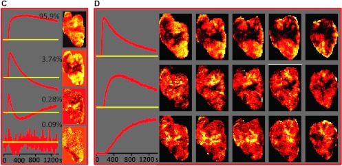
Analysis workflow illustrated for DCE-MRI data from a Dunning R3327-AT prostate tumor model. (A) A representative array of signal versus time curves from a tumor region and adjacent muscle tissue, depicted by the green box on a representative T₁-weighed MR image on the right, is shown. The color boxes indicate three differential temporal patterns in the tumor (from left to right): blue—continuous slow uptake; green—faster uptake and some washout; red—rapid contrast uptake and fast washout. On the basis of their temporal shape [6], as well as their image location, these curves are most likely associated with necrotic, hypoxic, and well-perfused tumors, respectively. (B) Left: First four PCs, together with their fractional contribution to the data variability. Right: Spatial distribution of the magnitude of the corresponding PC scores in the five image slices. (C) PCA applied only to the DCE data from pixels within the tumor. Left: First four PCs. Right: Spatial distribution of the magnitude of the corresponding PCs in a representative central tumor slice (note that the PCA was carried out on the entire data set). (D) cNMF analysis of the data seeking three solutions. Left: Basic signal versus time curves, S(t). Right: Spatial distribution of the corresponding weights, W, in the five tumor slices.