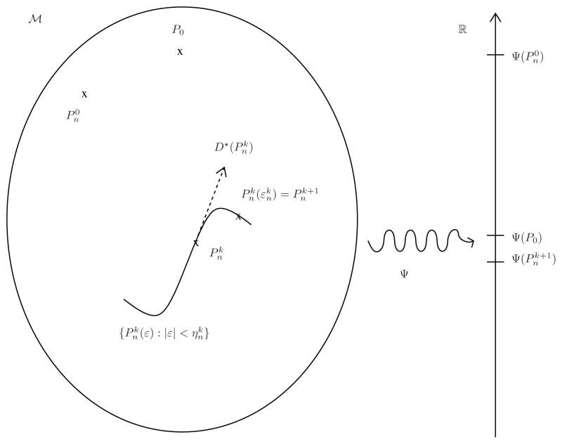
Fig 1.
Illustration of the TMLE procedure (with its general one-step updating procedure). We intentionally represent the initial estimator
closer to P0 than its kth and (k +1)th updates
and
, heuristically because
is as close to P0 as one can possibly get (given Pn and the specifics of the super-learning procedure) when targeting P0 itself. However, this obviously does not necessarily imply that
performs well when targeting Ψ (P0) (instead of P0), which is why we also intentionally represent
closer to Ψ (P0) than
. Indeed,
is obtained by fluctuating its predecessor
in the direction of Ψ ”, i.e., taking into account the fact that we are ultimately interested in estimating Ψ (P0). More specifically, the fluctuation {
} of
is a one-dimensional parametric model (hence its curvy shape in the large model
 ) such that (i)
, and (b) its score at ε = 0 equals the efficient influence curve
at
(hence the dotted arrow). An optimal stretch
is determined (e.g. by maximizing the likelihood on the fluctuation), yielding the update
.

