Abstract
Reconstruction of the past is an important task of evolutionary biology. It takes place at different points in a hierarchy of molecular variation, including genes, individuals, populations, and species. Statistical inference about population histories has recently received considerable attention, following the development of computational tools to provide tractable approaches to this very challenging problem. Here, we introduce a likelihood-based approach which generalizes a recently developed model for random fluctuations in allele frequencies based on an approximation to the neutral Wright–Fisher diffusion. Our new framework approximates the infinite alleles Wright–Fisher model and uses an implementation with an adaptive Markov chain Monte Carlo algorithm. The method is especially well suited to data sets harboring large population samples and relatively few loci for which other likelihood-based models are currently computationally intractable. Using our model, we reconstruct the global population history of a major human pathogen, Streptococcus pneumoniae. The results illustrate the potential to reach important biological insights to an evolutionary process by a population genetics approach, which can appropriately accommodate very large population samples.
Keywords: population history, genetic drift, infinite alleles Wright–Fisher model
Introduction
Phylogenetic analysis has become a central component of biology, maturing from simple analyses of presences and absences of morphological characters in the early days to today’s sophisticated mathematical and computational machinery that aims to infer the course a particular evolutionary process has taken place, from molecular observations. Because evolutionary processes happen at various levels of a hierarchy of molecular variation, including genes, individuals, populations, and species, the models need to be adapted to the specific purpose at hand. In contrast to standard models for phylogenetic inference, models for reconstructing population histories from molecular data have remained somewhat overshadowed, at least partly due to the computational challenges associated with a likelihood-based inference in this context. These challenges arise from a multitude of processes, including genetic drift, mutation, and migration, that shape the genetic variation in present-day populations.
When attempting to reconstruct population histories, the focus is on the need to model population trees, which might differ considerably from gene trees (Pamilo and Nei 1988; Maddison 1997; Degnan and Rosenberg 2009). From a population genetics perspective, coalescent theory provides in principle the necessary framework for specification of probabilities to the observed outcomes of combined evolutionary and demographic process (Ewens 2004; Hein et al. 2005). However, despite considerable computational advances, coalescent-based likelihood inferences remain in practice intractable when large population samples are observed (Wilson et al. 2003; Cornuet et al. 2008; RoyChoudhury et al. 2008; Heled and Drummond 2010; Bryant et al. 2012).
Alternatively, the population tree inference may be carried out by approximating changes in allele frequencies using diffusion approximations (Ewens 2004). Because the sufficient statistics emerging under such a model correspond to the counts of alleles observed in different populations, instead of individual genotypes, even very large samples from the populations can be efficiently handled in terms of computational complexity. The first such methods were introduced in the 1960s and 70s (Edwards and Cavalli-Sforza 1964; Cavalli-Sforza and Edwards 1967; Felsenstein 1973; Thompson 1975; Felsenstein 1981). They are based on approximating the diffusion limit of a Wright–Fisher model with Brownian motion after a suitable transformation of the frequencies. A similar model was introduced also by Nicholson et al. (2002) for assessing the level of differentiation in structured population, but it considered only star-shaped trees for the history of populations.
A related diffusion-based approximation for inferring the demographic history of multiple populations was proposed by Gutenkunst et al. (2009). They compute numerically the expected joint frequency spectrum with a biallelic Wright–Fisher diffusion, extending earlier work by Williamson et al. (2005) to multiple populations. The numerical approximation to the diffusion is computationally intensive and limited to at most three populations.
We recently introduced an approximation to the neutral Wright–Fisher diffusion model for allele frequencies at unlinked single nucleotide polymorphism (SNP) loci using a Bayesian hierarchical modeling approach (Sirén et al. 2011). It is based on the univariate Balding–Nichols model, which was originally developed in the context of equilibrium under migration and genetic drift in island populations, but currently widely used for modeling the effects of genetic drift on allele frequencies in subdivided populations (Balding and Nichols 1995; Falush et al. 2003; Gaggiotti and Foll 2010). The model applies to situations where the main source of variation between populations is genetic drift, that is, random fluctuations in allele frequencies occurring through demographic processes. It was therefore explicitly assumed that the genetic variation observed in the current populations had been present already in the common ancestral population, and consequently, the possibility that novel mutations have arisen following the split of the ancestral population was ignored.
Here, we generalize the pure drift model to account for the effect of mutations by deriving a corresponding approximation to the infinite alleles Wright–Fisher model (Kimura and Crow 1964; Ewens 2004). The model is derived for situations where genetic drift is the main source of genetic variation between populations, but the effects of mutations can not be ignored. As a special case of the model, a multi-allelic version of our earlier pure drift model for SNP loci arises, when the mutation rate is set equal to zero. To make statistical inference about the model parameters and the evolutionary distances between populations, we have implemented an adaptive Markov chain Monte Carlo (MCMC) algorithm to generate samples from the posterior distribution. Using the introduced framework, we reconstruct the global population history of a major human pathogen, Streptococcus pneumoniae. This illustrates well the potential of our approach to provide important biological insights to an evolutionary process by a population genetics approach that can appropriately accommodate very large population samples.
Materials and Methods
Statistical Model
We consider a setting where individuals are sampled from K distinct populations and genotyped at L unlinked loci to allow for inference about the history of the populations. The genetic relatedness of the populations is described by a rooted bifurcating tree topology T representing the order of divergence from a common ancestral population. The leaves of the topology T correspond to the K populations, whereas the inner nodes correspond to ancestral populations. Each branch c of T is associated with two parameters characterising the population between split events: number of generations tc and effective population size Nc. When written without the subindices, we refer to these two quantities in general, without reference to a particular pair of populations.
Let x denote the n × L matrix of genotypes of the sampled individuals at L unlinked loci, where n is the sum of the sample sizes from the K populations. Throughout this work, we consider only haploid organisms, but our model can equally well handle any ploidity with the parameters transformed accordingly. We let  denote the allele observed at locus l on row i in
  Presence of alleles missing at random in x will be appropriately taken into account in the likelihood introduced later, however, in order not to unnecessarily complicate the notation, we abstain from an explicit specification of the locations of any missing data elements.
We assume that the genetic variation within each locus can be modelled with a neutral infinite alleles model (Kimura and Crow 1964). The main consequences of this are that the alleles are represented by positive-valued integer codes instead of sequence level variation and that every mutation event creates a novel allele. The model is based on a diffusion approximation to the transition density of a neutral infinite alleles Wright–Fisher model, whose properties have been the subject of extensive study (Watterson 1976; Griffiths 1979b; Ethier and Kurtz 1981). However, most of the research has concentrated on the unlabeled version of the diffusion, where the allele frequencies are ordered in descending order, and which is less suitable for the analysis of multiple populations. Griffiths (1979a) derives exact sampling distributions for a number of scenarios, including a transient population and two populations having a common ancestral population. The results under the latter scenario have later been generalized by Watterson (1985) and Padmadisastra (1987). These results could in principle be generalized to any number of populations, but the exact formulae are complicated even for three populations.
A model for the change of the allele frequencies along the population tree T is built by assuming that each locus evolves independently of the other loci given the parameters t, N, and a mutation rate u. As stated earlier, each branch c of the tree is associated with parameters tc and Nc, but the mutation rate u is assumed to be common to all branches. This does not constrain the model as only two parameters or combinations of them are identifiable in each branch under the infinite alleles Wright–Fisher model. We use the relative time  and effective mutation parameter mc = uNc for each branch c in our model. The effective mutation parameter is related to the mutation parameter θ = 2uN (or θ = 4uN if the effective population size is 2N) commonly used in population genetics, but we have chosen not to use θ as it seems to be only partially identifiable.
Later, we simplify the notation by omitting reference to any particular locus, as the same processes are applied to the frequencies at all loci. The model extends the model introduced in Sirén et al. (2011) by allowing for loci with multiple alleles and letting mutation change the allele frequencies in addition to the genetic drift. For the details of derivation of the approximation and the relation to the Wright–Fisher model, see the Appendix.
Let S denote the set of alleles that were present with a positive frequency in the root population and let P denote those alleles that are not shared and have been created by mutation at some point in the tree. The alleles in S are shared indicating that they can have a nonzero frequency in all of the K leaf populations, whereas the alleles in P are private in the sense that they may only be observed within a subtree of T. Such a division of the alleles is motivated by the notion that the frequencies of shared alleles contain all the information about the divergence times between populations under the infinite alleles model (Griffiths 1979a). Note that the division of alleles into the sets S and P is unknown, because samples are available only for the leaf populations, but here we build the model conditionally on them. Different strategies to estimate the division are discussed along with other computational issues.
Each population node c of T, either observed or ancestral, is associated with the frequencies ψSc and ψPc of alleles in S and P, respectively. Here  is a vector of (relative) frequencies for the r alleles in S and ψPc is a scalar of the total (relative) frequency of alleles in P, so that
  . Using the standard definition in population genetics, ψSc and ψPc are referred to as allele frequency parameters and allele counts will be used to denote empirically observed abundances of alleles within a population sample. By definition,
  equals zero for the root population ca.
To approximate the dynamics of the Wright–Fisher diffusion process, we use a two-step Beta-Dirichlet model for the allele frequencies. For each node c except the root, the conditional distribution of the frequency of the private alleles ψPc given the frequency  in the parent node pa(c) is defined as
| (1) |
where μPc is the expectation of the distribution and ϕPc controls the variance, which is given by
 |
The frequencies of the shared alleles ψSc have the conditional distribution
| (2) |
where again μScj is the expectation and ϕSc controls the variance. The Beta-Dirichlet model is a natural generalization of the Dirichlet models widely used in the literature for markers without mutation (Falush et al. 2003; Gaggiotti and Foll 2010). The parameters of the earlier two distributions are chosen as
| (3a) |
 |
(3b) |
 |
(3c) |
| (3d) |
to yield the same expectation and covariance structure as obtained under the Wright–Fisher infinite alleles model. Unfortunately, the complicated form of the parameters does not provide any clear intuition about the dynamics of the model. See Appendix for the properties of these distributions and their relation to the Wright–Fisher model. For the frequencies  in the root population ca, we assume a uniform distribution.
It should be noted that the Wright–Fisher model we are approximating is time-reversible, which implies that the placement of the root along the branches of the tree is not identifiable. The root node in our model should preferably be interpreted as an auxiliary parameter and any indication about the placement of the root should be viewed as an artefact arising from the approximations used.
Assuming linkage equilibrium and that the genotyped individuals represent a random sample from each of the K populations, a product multinomial distribution is obtained for the allele counts conditionally on the allele frequencies, such that
 |
(4) |
where  is the joint multinomial probability of the allele counts
  at locus l in sample population c, with the allele frequencies now being indexed by the locus. Notice that the remaining parameters in (1) and (2) are assumed to be constant over the loci.
The earlier expressions for conditional distributions determine jointly a hierarchical model for the genotype data, which reflects the degree of genetic relatedness among the sample populations through the tree topology and the branch length parameters. Our model can be completed with a Bayesian formulation by assigning prior distributions to all the unknown parameters. When analyzing real data, the prior distributions can be chosen to reflect background information about the quantities that the parameters represent. However, in this work, we have simply used uniform distributions on the interval (0, 1) for the time parameters τ and exponential distributions with mean 1 for the relative mutation parameters m. These choices have been made to specify weakly informative prior distributions and they should not have any considerable effect on the resulting posterior inferences. The exponential distribution for the mutation parameters is ensuring that the parameter stays within a realistic range, as it might be weakly identifiable for some data sets. Finally, the tree topologies would typically be assigned a uniform prior distribution as is done more generally in Bayesian phylogenetics.
Computation
We have implemented an Adaptive Metropolis (AM) algorithm (Haario et al. 2001) to generate samples from the conditional posterior distribution of τ, m, and ψ, given a topology T and the partition of the alleles to sets P and S. An adaptive MCMC algorithm (Robert and Casella 2004) provides in general a much more efficient approach to approximating posterior distributions than a standard Metropolis–Hastings algorithm, when parameters are moderately or strongly correlated and the correlation structure is unknown. The essence of the AM algorithm is that the covariance matrix of the Gaussian proposal distribution is modified during the algorithm run based on the previous iterations, such that an adequate level of mixing is acquired in the resulting Markov chain. In our implementation, the parameters τ and m are updated jointly, whereas the allele frequencies ψ are updated separately for each locus and population node. All of the variables are transformed with logarithm or logit functions before applying the Gaussian proposals.
Inference about the tree topology T poses a more difficult computational challenge than the continuous parameters of the model. Ideally, one would like to assign prior distribution on the topologies and then make inferences from the corresponding posterior distribution by utilizing algorithms like the reversible jump MCMC (RJMCMC, Green 1995). However, because the parameter spaces associated with the topologies are partially different, the design of an efficient algorithm is more complicated. Moreover, the adaptivity of our AM algorithm would be lost in an RJMCMC algorithm and, consequently, it would be much more computationally expensive without a careful tuning of proposal distributions. Alternatively, it is possible to compute approximate marginal likelihoods from the output of MCMC for each potential topology, or calculate approximate Bayes factors for pairs of them (Newton and Raftery 1994; Kass and Raftery 1995; Han and Carlin 2001; Lartillot and Philippe 2006).
Instead of approximating posterior probabilities for topologies through marginal likelihood estimates calculated from the MCMC output, we have adopted in our numerical analyses a different approach similar to those widely used methods in phylogenetics that are based on estimating the evolutionary distances between pairs of taxa, which is considerably simpler regarding the computational effort. First, the AM algorithm is used separately on each pair of sampled populations. Second, we then compute the distance between the two populations as the sum of relative times τ because the divergence from a common ancestral population. Finally, we construct the tree topology by finding the unrooted binary tree using the least squares criterion (see Felsenstein 2004, Chapter 11). As we do this separately for each sample obtained from the posterior distribution of the pairwise distances, we get a measure of statistical uncertainty associated with the topology by counting the relative number of times each topology is the minimum scoring tree. Conditional on any topology constructed in this manner, one can obtain posterior inferences for its branch lengths directly from the MCMC samples by including the fraction of samples leading to the particular topology.
In all of our analyses, the partition of the alleles to shared and private was based on the observed alleles. If an allele was observed in only a single population, it was assumed to be private and otherwise shared. We tried other possibilities for dividing the alleles, which could take the tree topology into account, but they provided inferior results compared to this choice.
Results
Analysis of Simulated Data
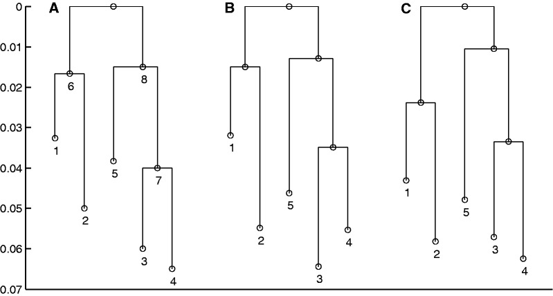
To test the validity of our model for inference in population phylogenies, we simulated data using the Wright–Fisher infinite alleles model. The topology of the tree along with the population sizes and numbers of generations are shown in figure 1A and table 1. The mutation rate was fixed to  for all loci leading to an effective mutation parameter m in the range 0.5–1.5. Allele frequencies were simulated for 112 loci. The allele frequencies in the root population were generated by simulating the Wright–Fisher model for
  generations in a population of 105 individuals from a starting point with 10 alleles at uniform frequencies. This ensured that the distribution of frequencies in the root was close to the stationary distribution. For each of the populations, a sample of 200 alleles was taken at each locus.
Fig. 1.
Correct and estimated branch lengths for the simulated data set. The length of each branch is proportional to the value of corresponding relative time τ parameter. (A) Values used in simulation, (B) posterior expectations from analysis using 7 loci, and (C) 112 loci.
Table 1.
Parameter Values Used for the Simulated Data.
| Brancha | N | T | τ |
|---|---|---|---|
| 1 | 2.5 × 10⁴ | 400 | 0.016 |
| 2 | 1.5 × 10⁴ | 500 | 0.033 |
| 3 | 1.5 × 10⁴ | 300 | 0.02 |
| 4 | 1 × 10⁴ | 250 | 0.025 |
| 5 | 3 × 10⁴ | 700 | 0.023 |
| 6 | 3 × 10⁴ | 500 | 0.017 |
| 7 | 1 × 10⁴ | 250 | 0.025 |
| 8 | 2 × 10⁴ | 300 | 0.015 |
aNumber refers to the child node of the branch.
We analyzed the simulated data with the number of populations considered simultaneously varying between 2 and 5. First, we estimated the pairwise distances between each pair of populations. These were obtained by running the MCMC sampler with the corresponding populations and summing the distances τ to the root. The number of loci used varied between 7 and 112. In this and other analyses, we ran two independent chains for each combination of populations and number of loci to ensure that the sampler converged properly. In all cases, the sampler was run for 5 × 10⁵ iterations with the first 105 iterations used as burn-in. The chains were further thinned by collecting every 40th sample to get 104 posterior samples for the estimation. The runtime of a single chain for analysis of 7 loci was approximately 50 min using a single core of a 2.6 GHz AMD Opteron processor. For larger number of loci, the running time scaled linearly.
Figure 2 shows the posterior distributions of the pairwise distances with varying number of loci. We note that the pairwise distances are underestimated even with 112 loci and the 50% posterior intervals do not include the correct values. This is most likely due to the way of dividing the alleles into private and shared, as it does not take account the possibility that an ancestral allele might disappear from one of the populations. In such cases, our procedure assumes wrongly that it is a novel mutation. Nevertheless, the ratio of estimated distances with 112 loci to the correct values is in the range 0.8–0.91 for all pairs of populations. Hence, the distance seem to converge to the truth relative to each other, but the absolute values are somewhat biased. The pairwise distances were also used to infer the correct topology with the least squares approach described earlier. Using 7 and 14 loci the correct unrooted topology was recovered in 99.24% and 99.99% of the cases, respectively. With 28 or more loci, the best tree had the correct topology in all of the posterior samples.
Fig. 2.
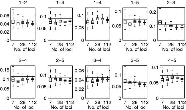
Posterior estimates of the pairwise distances with different number of loci. Box plots of the posterior distributions for sum of distances to the root τ for each pair of populations from the analysis of the simulated data. The number of loci used was 7, 14, 28, 56, and 112. The pair of populations is indicated above each subplot. The box depicts the 25% and 75% quantiles and the whiskers depict the minimum and maximum among posterior samples. The horizontal line depicts the value used in simulating the data.
Next, we analyzed all of the populations simultaneously with the correct tree topology using between 7 and 112 loci. The AM algorithm was again run for  iterations with the first 105 iterations used as burn-in. Figure 1B and C show the posterior means of the branch lengths with 7 and 112 loci, respectively. Figure 3 shows the posterior means of the branch lengths as functions of the number of loci used along with the correct values. The estimates seem to get reasonably close to the correct values in all other cases except for the branch connecting population 5. The length of this branch is the most difficult one to estimate because the parent node of population 5 does not have another observed population as a child.
Fig. 3.
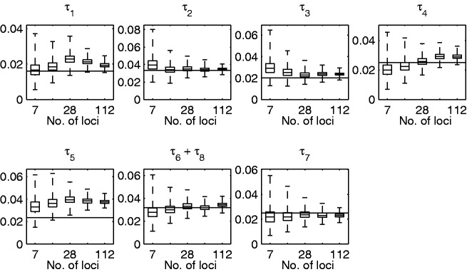
Posterior estimates of the branch lengths with different number of loci. Box plots of the posterior distributions for the branch lengths τ from the analysis of the simulated data using the correct topology. The number of loci used was 7, 14, 28, 56, and 112. The box depicts the 25% and 75% quantiles and the whiskers depict the minimum and maximum among posterior samples. The lengths of the two branches 6 and 8 connected to the root are summed, because the placement of the root is not identifiable under the infinite alleles model. The horizontal line depicts the value used in simulating the data.
We also analyzed two subtrees with populations (3, 4, 5) and (1, 2, 3, 4). The distributions of branch length estimates with varying number of loci are shown in supplementary figures S1 and S2, Supplementary Material online. These estimates appear to be much closer to the correct ones than in the pairwise case or with all the populations simultaneously.
Analysis of S. pneumoniae
Streptococcus pneumoniae is a major human pathogen responsible for over 1 million deaths each year (O’Brien et al. 2009). Colonization is the normal state in the life history of S. pneumoniae, and disease only a rare outcome. Depending on the sample, between 20% and 80% of individuals are carrying S. pneumoniae asymptomatically at any time. Historically, S. pneumoniae has been divided into strains by serotype. Serotyping is a means of classification that uses the major surface antigen of the bacterium to divide the population into 93 strains. Geographic differences in the serotype composition of the S. pneumoniae population were noted as early as 1931, when Milam and Smillie investigated the strains isolated from an isolated tropical island (St. John, in the United States Virgin Islands) and found them to be distinct from those circulating in New York City (Milam and Smillie 1931). More recently, these differences have been studied in detail. In general, the pneumococcal populations in Europe and the United States are quite similar to one another in terms of serotype composition, and distinct from the populations in South America, Asia, and Africa. The latter are similar to each other and characterized by a higher prevalence of certain serotypes such as 1, 2, and 5 that are rare in European and North American settings (Hausdorff et al. 2001).
Serotype has more recently been augmented by the greater resolution offered by molecular epidemiology. Multi-locus sequence typing (MLST, Enright and Spratt 1998) is a commonly used typing method that genotypes strains at seven loci. We wished to test whether the MLST data would support the geographical structuring previously described (Hausdorff et al. 2001), and whether any geographically defined populations are more divergent and distinctive than others. Genotypes of isolates from samples collected worldwide are publicly available in the MLST database at URL http://spneumoniae.mlst.net/ (last accessed February 1, 2011). The MLST database contains allelic data for the following seven housekeeping genes: aroE, gdh, gki, recP, spi, xpt, and ddl. Using data from Africa accessed on February 1, 2011, we reconstructed the intra-continental population history, based on three local populations representing East (347 isolates), South (388 isolates), and West Africa (1,130 isolates). For each local population, the data were almost exclusively derived from a single country. With these sample populations, there are three possible rooted topologies and the MCMC sampler was used to generate posterior samples of the parameters for each of them. We ran two independent chains of 106 iterations for each topology to ensure that the MCMC sampler had properly converged. The chains were thinned by collecting every 80th sample, with  initial samples excluded as burn-in. As expected, no differences appeared among the rooted topologies, due to the time reversibility of the underlying infinite alleles model, and the independent runs resulted in practically identical results for each topology. Posterior summaries of the model parameters are given in figure 4 for one of the three rooted topologies.
Fig. 4.
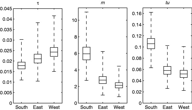
Posterior estimates of the parameter values for the African Streptococcus pneumoniae populations. Box plots of the posterior distributions for the relative time τ, the effective mutation rate m and the product tu. The box depicts the 25% and 75% quantiles and the whiskers depict the minimum and maximum among posterior samples.
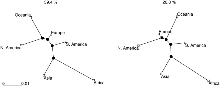
To reconstruct the global population history of S. pneumoniae, we considered each continent as a sample population, with the following numbers of isolates available in the database (data accessed on February 1, 2011): Africa (1,981), Asia (1,553), Europe (5,029), Oceania (168), South America (526), and North America (1,664). Here, we used the pairwise approach based on 106 iterations, thinned to every 80th sample, with  initial samples discarded as burn-in. For each pair of populations, we ran two independent MCMC chains and obtained indistinguishable results, indicating that the sampler had converged properly. Trees were constructed from 10,000 final posterior samples and the two most frequent topologies are shown in figure 5. Posterior expectations and 95% posterior intervals of the pairwise distances are given in table 2. We also generated a phylogenetic network in SplitsTree4 (Huson and Bryant 2006) to visualize the relationships between populations. The network was created from the posterior expectations of the pair-wise distances using the neighbor-net method (Bryant and Moulton 2004) and is shown in figure 6.
Fig. 5.
Trees with most support from the pair-wise analysis of global Streptococcus pneumoniae populations. Two tree topologies with most support. The percentage above each tree shows the proportion of the posterior samples for which the corresponding had best fit. The branch lengths are averages from the posterior samples.
Table 2.
Posterior Expectations (lower triangle) and 95% Posterior Intervals (upper triangle) for Pairwise Distances of Global Streptococcus pneumoniae Populations.
| Africa | Asia | Europe | Oceania | South America | North America | |
|---|---|---|---|---|---|---|
| Africa | — | 0.03–0.043 | 0.032–0.046 | 0.042–0.067 | 0.027–0.042 | 0.044–0.065 |
| Asia | 0.036 | — | 0.021–0.031 | 0.028–0.045 | 0.025–0.039 | 0.028–0.042 |
| Europe | 0.039 | 0.064 | — | 0.015–0.026 | 0.013–0.021 | 0.013–0.021 |
| Oceania | 0.054 | 0.06 | 0.02 | — | 0.02–0.035 | 0.021–0.036 |
| South America | 0.034 | 0.032 | 0.017 | 0.027 | — | 0.021–0.033 |
| North America | 0.054 | 0.034 | 0.017 | 0.028 | 0.026 | — |
Fig. 6.
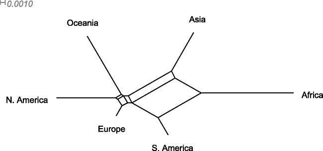
Phylogenetic network from the pair-wise analysis of global Streptococcus pneumoniae populations. The network was generated in SplitTree4 program using posterior expectations of the branch lengths as the distances.
Extensive network structure is evident, with poor resolution of the specific branching patterns of the continental subpopulations. We suggest that this reflects recent migration. The length of the branches in figure 6 reflects drift, and hence the amount of unique diversity accumulated in each population. Even with extensive migration, the African samples are plainly highly divergent. Contrastingly, the European sample lies at the end of a very short branch, possibly reflecting concentrated sampling of this region in the database, and extensive migration between this region and the rest of the world.
Although the network shown in figure 6 reflects conflicting signal, it does not preferentially weight those relationships that are most well supported by the data. The two topologies most frequently sampled from the posterior are shown in figure 5. These clearly support the distinct nature of the populations found in South America and Asia, as previously reported (Hausdorff et al. 2001), and also provides strong evidence for the divergence of the African population consistent with recent observations of the sequence variation in the largest African carriage sample published to date (Donkor et al. 2011). The North American, European, and Oceanian populations are clearly closely related, and the only difference between the two topologies is in the grouping of these populations, possibly reflecting conflicting signal arising from frequent intercontinental travel. However, it is consistent with the observations regarding serotype compositions on different continents referred earlier.
Discussion
Our likelihood-based method provides a considerable generalization over the purely drift-based model introduced in Sirén et al. (2011), extending the approach to data where the effect of mutation needs to be explicitly considered. We demonstrated the usefulness of this approach by an application to a major human pathogen, S. pneumoniae, showing the clearly divergent nature of the population circulating in Africa from all other samples a distinction that was obscure using historical serotyping data. We also found in our pairwise analysis considerable evidence for phylogenetic inconsistency, as displayed graphically in figure 6, in particular among the North American, European, and Oceania populations.
In the analysis of simulated data, the posterior estimates of the parameters converged close to the correct values in most cases, but some bias is evident in others. It should be noted that the data were simulated under the exact Wright–Fisher infinite alleles model, whereas our method is based on approximating a truncated version of its diffusion approximation, and, therefore, minor bias in the results is expected. Another source of possible bias is also the partitioning of the alleles into the sets S and P. As the partition is obtained by comparing the observed numbers of alleles in each population outside the model, we are effectively modeling a conditional version of the diffusion. This conditioning might change the dynamics of the diffusion in a way which could result in biased estimates, although we have not studied it in detail. However, we believe that the approach used in this work should not cause any serious bias, as is shown by the analysis of simulated data.
The model described here could be extended in several directions. For example, the partitioning of the alleles into shared and private could be included in the model. This could in principle be achieved by utilizing generalizations to Dirichlet distributions used in Bayesian nonparametrics (Hjort et al. 2010). Also, the sampling model used in our study was assumed to be basic random sampling, which may not always be adequate, in particular for bacterial data from clinically important organisms. Therefore, other sampling designs could be considered and easily used with the corresponding likelihood functions to extend the basic model.
Homologous recombination is a factor which needs to be considered when modeling the evolution of many named bacterial species. The extent to which recombination affects inference will largely depend on the geographical scale of the analysis. Recombination can cause difficulties in particular under two different circumstances. First, when recombination has occurred between different parts of the tree, the data deviate from the vertical process of evolution in the allele frequencies. When each locus is considered independently, then recombination between populations is effectively equal to migration event. It should be noted though that recombination within a population only weakens linkage disequilibrium between loci, if whole gene sequences are transferred. In addition, novel alleles brought by recombination from some unsampled outgroup can be adequately modelled in terms of mutation (as they generate new alleles). Note that this would not be the case with explicit modelling of sequence evolution, in contrast to the infinite alleles assumption used here. Second, when recombination affects only a part of a single gene sequence, novel alleles are likely to be generated. How well a mutation model can approximate this effect remains unknown, but it will depend on the ratio of mutation to recombination rate for the species in question. However, the direct effect will follow from how often a recombination has replaced a segment in the genome, which is not expected to be very frequent for few short segments such as those considered in the MLST data. Estimates of mutation parameters may be biased by these factors. The extent to which this is the case is a subject of ongoing research.
A full model-based approach would be preferable for inferring tree topologies instead of the estimation of pairwise evolutionary distances as pursued here. However, it is inevitably computationally more expensive than the current approach, which at its present form requires considerable computational resources. We target to explore these possibilities closer in future and also examine the accuracy of approximations to marginal likelihood based on posterior samples of parameters conditional on a fixed topology. One possibility could be to include the method as a part of an existing phylogenetic software package such as BEAST (Drummond and Rambaut 2007), which already implements sophisticated algorithms for traversing the space of trees. A free software package implementing both the pure drift and infinite alleles models is available for download at URL http://www.helsinki.fi/bsg (last accessed November 6, 2012).
Supplementary Material
Supplementary figures S1 and S2 are available at Molecular Biology and Evolution online (http://www.mbe.oxfordjournals.org/).
Acknowledgments
This work benefited significantly from the comments of three anonymous reviewers and from the discussions with participants of the 2nd Permafrost Workshop. This work was supported by Finnish Doctoral Programme in Computational Sciences FICS, Academy of Finland grant no. 251170 (Finnish Centre of Excellence Program (20122017)), and European Research Council grant no. 239784. W.P.H. was supported by funding from NIH/NIGMS GM088558-01 for the MIDAS Center for Communicable Disease Dynamics at HSPH.
Appendix
Consider a locus with r alleles following Wright–Fisher model in a population with fixed size N. Assume that the r − 1 first alleles mutate to the rth type at rate m/N and no other mutations occurs. This can be seen as a truncated version of an infinite alleles model, where the r − 1 first alleles are followed and the rth allele includes all other alleles. Let Xjt and  , denote the number and the relative frequency of allele j at generation t. In this model, the alleles at generation t are obtained as a random sample with replacement from the previous generation t − 1. The numbers of different alleles have a multinomial distribution conditional on the alleles of the previous generation
where ηt is a r dimensional vector with entries
 |
Conditional on the frequency ψr0 we get the expectation of ψrt as
by using the rule of iterated expectation. Now letting t and N go to infinity so that t/N → τ the expectation becomes
| (5) |
where with slight abuse of the notation ψrτ refers to the frequency at generation τN.
The conditional variance of ψrt given ψr0 is obtained by recursive application of the variance decomposition as
 |
Assuming t and N large, this may be approximated as an integral
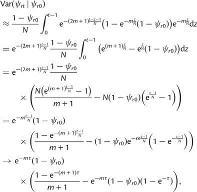 |
(6) |
as N, t → ∞ and tN →τ.
The conditional mean and variance of ψjτ are easily obtained for  , as ψjτ behaves like 1 − ψrτ. Thus
 |
Using similar techniques as with the variance, we can compute the conditional covariance between ψjτ and  , as
, as
and the conditional covariance between ψjτ and ψrτ as
 |
Consider now the Beta-Dirichlet model specified in equations (1) and (2) with parameters (3). We show that this model has same expectations and covariances as the model described earlier. As ψPc follows a Beta distribution it has expectation
and variance
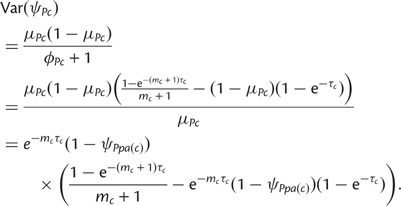 |
In the earlier mentioned and following equations, we have dropped the conditioning to ψPpa(c) and ψSpa(c) to simplify the notation. For  , we have
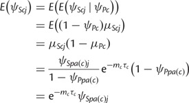 |
and
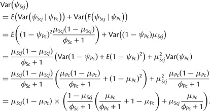 |
Plugging in the parameter values, the expression for variance becomes
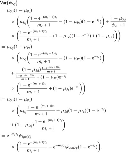 |
The covariance between shared and private alleles has the form
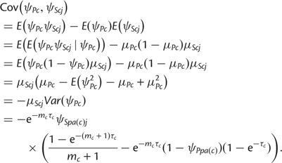 |
Finally, the covariance between ψSck and  , is given by
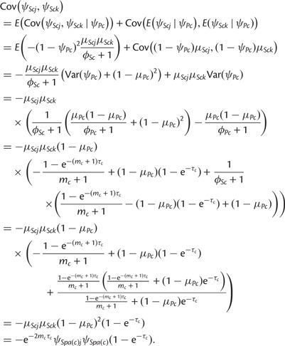 |
References
- Balding DJ, Nichols RA. A method for quantifying differentiation between populations at multi-allelic loci and its implications for investigating identity and paternity. Genetica. 1995;96:3–12. doi: 10.1007/BF01441146. [DOI] [PubMed] [Google Scholar]
- Bryant D, Bouckaert R, Felsenstein J, Rosenberg N, RoyChoudhury A. Inferring species trees directly from biallelic genetic markers: bypassing gene trees in a full coalescent analysis. Mol Biol Evol. 2012;29:1917–1932. doi: 10.1093/molbev/mss086. [DOI] [PMC free article] [PubMed] [Google Scholar]
- Bryant D, Moulton V. Neighbor-net: an agglomerative method for the construction of phylogenetic networks. Mol Biol Evol. 2004;21:255–265. doi: 10.1093/molbev/msh018. [DOI] [PubMed] [Google Scholar]
- Cavalli-Sforza L, Edwards A. Phylogenetic analysis: models and estimation procedures. Am J Hum Genet. 1967;19:233–257. [PMC free article] [PubMed] [Google Scholar]
- Cornuet JM, Santos F, Beaumont MA, Robert CP, Marin JM, Balding DJ, Guillemaud T, Estoup A. Inferring population history with DIY ABC: a user-friendly approach to approximate Bayesian computation. Bioinformatics. 2008;24:2713–2719. doi: 10.1093/bioinformatics/btn514. [DOI] [PMC free article] [PubMed] [Google Scholar]
- Degnan J, Rosenberg N. Gene tree discordance, phylogenetic inference and the multispecies coalescent. Trends Ecol Evol. 2009;24:332–340. doi: 10.1016/j.tree.2009.01.009. [DOI] [PubMed] [Google Scholar]
- Donkor ES, Bishop CJ, Antonio M, Wren B, Hanage WP. High levels of recombination among Streptococcus pneumoniae isolates from the Gambia. MBio. 2011;2:e00040–11. doi: 10.1128/mBio.00040-11. [DOI] [PMC free article] [PubMed] [Google Scholar]
- Drummond A, Rambaut A. Beast: Bayesian evolutionary analysis by sampling trees. BMC Evol Biol. 2007;7:214. doi: 10.1186/1471-2148-7-214. [DOI] [PMC free article] [PubMed] [Google Scholar]
- Edwards A, Cavalli-Sforza L. Reconstruction of evolutionary trees. In: Heywood V, McNeill J, editors. Phenetic and phylogenetic classification. London: Systematics Association. Publication; 1964. No. 6, p. 67–76. [Google Scholar]
- Enright MC, Spratt BG. A multilocus sequence typing scheme for Streptococcus pneumoniae: identification of clones associated with serious invasive disease. Microbiology. 1998;144:3049–3060. doi: 10.1099/00221287-144-11-3049. [DOI] [PubMed] [Google Scholar]
- Ethier S, Kurtz T. The infinitely-many-neutral-alleles diffusion model. Adv Appl Probab. 1981;13:429–452. [Google Scholar]
- Ewens W. Mathematical population genetics: theoretical introduction. New York: Springer; 2004. [Google Scholar]
- Falush D, Stephens M, Pritchard JK. Inference of population structure using multilocus genotype data: linked loci and correlated allele frequencies. Genetics. 2003;164:1567–1587. doi: 10.1093/genetics/164.4.1567. [DOI] [PMC free article] [PubMed] [Google Scholar]
- Felsenstein J. Maximum-likelihood estimation of evolutionary trees from continuous characters. Am J Hum Genet. 1973;25:471. [PMC free article] [PubMed] [Google Scholar]
- Felsenstein J. Evolutionary trees from gene frequencies and quantitative characters: finding maximum likelihood estimates. Evolution. 1981;35:1229–1242. doi: 10.1111/j.1558-5646.1981.tb04991.x. [DOI] [PubMed] [Google Scholar]
- Felsenstein J. Inferring phylogenies. Sunderland (MA): Sinauer Associates; 2004. [Google Scholar]
- Gaggiotti OE, Foll M. Quantifying population structure using the f-model. Mol Ecol Resour. 2010;10:821–830. doi: 10.1111/j.1755-0998.2010.02873.x. [DOI] [PubMed] [Google Scholar]
- Green P. Reversible jump Markov chain Monte Carlo computation and Bayesian model determination. Biometrika. 1995;82:711. [Google Scholar]
- Griffiths R. Exact sampling distributions from the infinite neutral alleles model. Adv Appl Probab. 1979a;11:326–354. [Google Scholar]
- Griffiths R. On the distribution of allele frequencies in a diffusion model. Theor Popul Biol. 1979b;15:140–158. [Google Scholar]
- Gutenkunst RN, Hernandez RD, Williamson SH, Bustamante CD. Inferring the joint demographic history of multiple populations from multidimensional SNP frequency data. PLoS Genet. 2009;5:e1000695. doi: 10.1371/journal.pgen.1000695. [DOI] [PMC free article] [PubMed] [Google Scholar]
- Haario H, Saksman E, Tamminen J. An adaptive metropolis algorithm. Bernoulli. 2001;7:223–242. [Google Scholar]
- Han C, Carlin B. Markov chain Monte Carlo methods for computing Bayes factors. J Am Stat Assoc. 2001;96:1122–1132. [Google Scholar]
- Hausdorff WP, Siber G, Paradiso PR. Geographical differences in invasive pneumococcal disease rates and serotype frequency in young children. Lancet. 2001;357:950–952. doi: 10.1016/S0140-6736(00)04222-7. [DOI] [PubMed] [Google Scholar]
- Hein J, Schierup MH, Wiuf C. Gene genealogies, variation and evolution. London/New York/Oxford: Oxford University Press; 2005. [Google Scholar]
- Heled J, Drummond AJ. Bayesian inference of species trees from multilocus data. Mol Biol Evol. 2010;27:570–580. doi: 10.1093/molbev/msp274. [DOI] [PMC free article] [PubMed] [Google Scholar]
- Hjort NL, Holmes C, Müller P, Walker SG, editors. Bayesian nonparametrics. Cambridge (UK): Cambridge University Press; 2010. [Google Scholar]
- Huson DH, Bryant D. Application of phylogenetic networks in evolutionary studies. Mol Biol Evol. 2006;23:254–267. doi: 10.1093/molbev/msj030. [DOI] [PubMed] [Google Scholar]
- Kass R, Raftery A. Bayes factors. J Am Stat Assoc. 1995;90:773–795. [Google Scholar]
- Kimura M, Crow J. The number of alleles that can be maintained in a finite population. Genetics. 1964;49:725–738. doi: 10.1093/genetics/49.4.725. [DOI] [PMC free article] [PubMed] [Google Scholar]
- Lartillot N, Philippe H. Computing Bayes factors using thermodynamic integration. Syst Biol. 2006;55:195. doi: 10.1080/10635150500433722. [DOI] [PubMed] [Google Scholar]
- Maddison WP. Gene trees in species trees. Syst Biol. 1997;46:523–536. [Google Scholar]
- Milam DF, Smillie WG. A bacteriological study of “colds” on an isolated tropical island (St. John, United States Virgin Islands, West Indies) J Exp Med. 1931;53:733–752. doi: 10.1084/jem.53.5.733. [DOI] [PMC free article] [PubMed] [Google Scholar]
- Newton MA, Raftery AE. Approximate Bayesian inference with the weighted likelihood bootstrap. J Roy Stat Soc B. 1994;56:3–48. [Google Scholar]
- Nicholson G, Smith AV, Jónsson F, Gústafsson O, Stefánsson K, Donnelly P. Assessing population differentiation and isolation from single-nucleotide polymorphism data. J Roy Stat Soc B. 2002;64:695–715. [Google Scholar]
- O’Brien KL, Wolfson LJ, Watt JP, Henkle E, Deloria-Knoll M, McCall N, Lee E, Mulholland K, Levine OS, Cherian T. Burden of disease caused by Streptococcus pneumoniae in children younger than 5 years: global estimates. Lancet. 2009;374:893–902. doi: 10.1016/S0140-6736(09)61204-6. [DOI] [PubMed] [Google Scholar]
- Padmadisastra S. The genetic divergence of three populations. Theor Popul Biol. 1987;32:347–365. [Google Scholar]
- Pamilo P, Nei M. Relationships between gene trees and species trees. Mol Biol Evol. 1988;5:568. doi: 10.1093/oxfordjournals.molbev.a040517. [DOI] [PubMed] [Google Scholar]
- Robert C, Casella G. Monte Carlo statistical methods. New York: Springer; 2004. [Google Scholar]
- RoyChoudhury A, Felsenstein J, Thompson EA. A two-stage pruning algorithm for likelihood computation for a population tree. Genetics. 2008;180:1095–1105. doi: 10.1534/genetics.107.085753. [DOI] [PMC free article] [PubMed] [Google Scholar]
- Sirén J, Marttinen P, Corander J. Reconstructing population histories from single nucleotide polymorphism data. Mol Biol Evol. 2011;28:673–683. doi: 10.1093/molbev/msq236. [DOI] [PubMed] [Google Scholar]
- Thompson E. Human evolutionary trees. Cambridge (UK): Cambridge University Press; 1975. [Google Scholar]
- Watterson G. The stationary distribution of the infinitely-many neutral alleles diffusion model. J Appl Probab. 1976;13:639–651. [Google Scholar]
- Watterson G. The genetic divergence of two populations. Theor Popul Biol. 1985;27:298–317. [Google Scholar]
- Williamson SH, Hernandez R, Fledel-Alon A, Zhu L, Nielsen R, Bustamante CD. Simultaneous inference of selection and population growth from patterns of variation in the human genome. Proc Natl Acad Sci U S A. 2005;102:7882–7887. doi: 10.1073/pnas.0502300102. [DOI] [PMC free article] [PubMed] [Google Scholar]
- Wilson IJ, Weale ME, Balding DJ. Inferences from DNA data: population histories, evolutionary processes, and forensic match probabilities. J Roy Stat Soc A. 2003;166:155–201. [Google Scholar]
Associated Data
This section collects any data citations, data availability statements, or supplementary materials included in this article.


