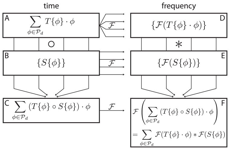
Figure 1. DFT–Convolution Theorem Modified for Partial-Component Subsampling.
Each hypercomplex component of the time-domain data (panel A) is subsampled by the corresponding component of the sampling function (panel B) according to the Hadamard product (∘) to produce zero-augmented, subsampled data (panel C). All quantities in the time domain (left column) are transformed to the frequency domain (right column) by the DFT (denoted by the horizontal arrows labeled with
 ). Each component of the time-domain data is isolated and processed by DFT, producing a set of hypercomplex spectra (indicated by the “one-to-many” grouping of arrows from panel A to panel D). Each of the real-valued sampling function components is processed by DFT to produce a set of hypercomplex PSFs (indicated by the set of disjoint arrows from panel B to panel E). The spectrum of the zero-augmented, subsampled data can be reached either by taking its DFT (indicated by the single arrow from panel C to panel F) or by pairwise convolving the set of uniformly sampled spectra with the PSF set and adding (indicated by the “many-to-one” grouping of arrows from panels D and E to panel F). The equivalence of these results (shown in panel F) is the modified DFT–Convolution relationship.

