Figure 4.

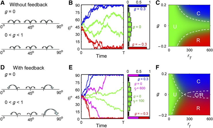
Stochastic modeling. Without feedback (A) Schematics showing the dependence of r_a and r_p on g. For g=0, r_a=r_p and for 0<g<1, r_a>r_p. Values of r_a and r_p do not depend on θ_a. (B) (Left) Stochastic simulation of θ_a from t=0 to t=T (division of P cell) (Right) Histograms of θ_a(T) for constant r_T=0.05 with different values of g=0.3 (blue), g=0 (green), and g=−0.3 (red). (C) Phase diagram showing the parameters space of g and r_f giving rise to correct polarity (blue/C), reverse polarity (red/R), and unpolarized divisions (green/U). Dotted lines show the region of parameter space giving rise to 35% correct polarity (top) or 35% reverse polarity (bottom). With feedback (D) Schematics showing the dependence of r_a and r_p on g and θ. For g=0, r_a=r_p at θ_a=45°. For 0<g<1, r_a>r_p at θ_a=45°. For both cases, r_a increases with θ_a whereas r_p decreases with θ_a. (E) (Left) Stochastic simulation of θ_a from t=0 to t=T (division of P cell) (Right) Histograms of θ_a(T) for g=0.3 and r_f=0.06 (blue), for g=−0.3 and r_f=0.06 (red), for g=0 and r_f=0.06 (magneta) and for g=0 and r_f=0.01 (green). (F) Phase diagram showing the parameters space of g and r_f giving rise to correct polarity (blue/C), reversed polarity (red/R), unpolarized divisions (green/U), and coexistence of correct and reverse polarity (magneta/C/R). Dotted lines show the region of parameter space giving rise to 35% correct divisions (top) or 35% polarity flips (bottom). The intersection of the two dotted lines shows the coexistence of correct and reverse polarity.