Figure 3.

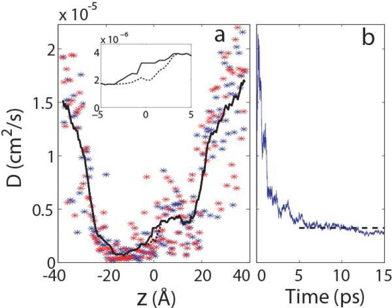
(a) The position-dependent diffusion coefficients D(z) , calculated from two sets of 1-ns umbrella sampling simulations with different initial coordinates.³³ The blue and red stars represent the local diffusion coefficients in each umbrella window obtained from the two simulations, respectively. The black dashed curve is the smoothed D(z) by applying moving average as described in the text. The black solid curve is obtained by using the optimal diffusion coefficient from (b) to update the D(z) values in the barrier region (highlighted in inset), as described in the text. (b) The optimal diffusion coefficient at the barrier top estimated from 200 unrestrained simulations. At each time step, the distribution of the ion coordinates is obtained from the corresponding snapshots in the 200 trajectories, and an optimal diffusion coefficient is then determined by maximizing the likelihood function L(D) (Eq. 25), as described in the text. The black dashed line indicates the average over the values between 5 ps and 15 ps, which is used to correct the D(z) curve in (a) at the barrier top.