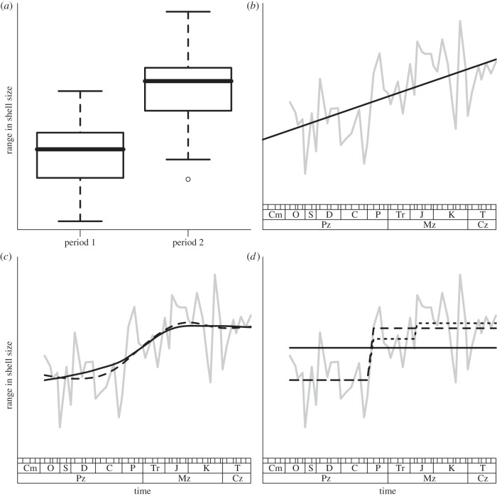
Figure 1.

Four ways of analysing trends in biodiversity. The data are range in gastropod fossil shell size (a metric of trait diversity) through the Phanerozoic from Kosnik et al. [8]. Similar figures analysing taxonomic and genetic diversity are included in the electronic supplementary material, figures S4 and S5 to illustrate how similar analysis tools can be used for different components of biodiversity. Grey lines show the observed data. All analysis done in R v. 2.12.2 (90); the code is included as electronic supplementary material. (a) t-test comparing shell size diversity in two time intervals (plotted as a box plot) with observed mean shell size range significantly different at p < 0.001. (b) Global trend analysis; a linear trend is fit using both ordinary least squares (OLS; which ignores the non-independence of errors close in time, black solid line), and generalized least squares (GLS) using a model with AR1 temporal autocorrelation of errors (dashed line). The two lines estimated by the two methods are identical; hence, only the solid line is visible. The main difference in the two models is for the p value with p = 0.007 for the OLS and the more conservative and correct value from the GLS of p = 0.033. (c) Local trend analysis; local regression using LOESS smoothing (black solid line) and a GAM spline model (dashed line) of richness versus time are plotted. The results are similar with both methods suggesting that the change in trait diversity over time is nonlinear. (d) Threshold regression [9] to formally identify both the number and location of breakpoints. The plot shows the null model of no threshold (black solid line), the preferred model of one threshold break (dashed line) and the second best model of two thresholds (pointed line). The preferred model shows a ΔBIC of >8 versus the null model showing very little evidence to select the null model. An F-test also shows the null model rejected at p < 0.001. Similar figures are included in the electronic supplementary material, using examples of genetic and taxonomic diversity on the y-axis.