Figure 5.

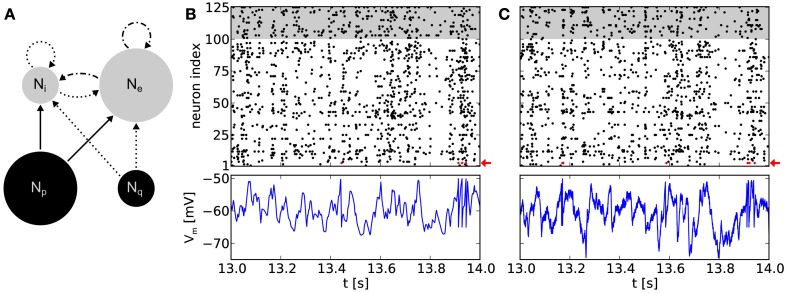
(A) Network topology of a balanced random network. Populations consisting of N_e = 100 excitatory and N_i = 25 inhibitory neurons (gray circles), respectively, are stimulated by populations of Poisson sources (black circles). We use N_p = 100 independent sources for excitation and N_q = 25 for inhibition. Arrows denote projections between these populations with connection probabilities p = 0.1, with solid lines for excitatory and dotted lines for inhibitory connections. Dot and dash lines are indicating excitatory projections with short-term depression. (B) Top: raster plot of a software simulation. Populations of excitatory and inhibitory neurons are depicted with white and gray background, respectively. Note that for clarity only the time interval [13 s, 14 s] of a 20 s emulation is shown. For the full 20 s emulation, we have measured C_V = 0.96 ± 0.09 (mean over all neurons) and C_C = 0.010 ± 0.017 (mean over 1000 random chosen pairs of neurons), respectively. Bottom: recorded membrane potential of an arbitrary excitatory neuron (neuron index 3, highlighted with a red arrow in the above raster plot). (C) Same network topology and stimulus as in (B), but emulated on the Spikey chip, resulting in C_V = 1.02 ± 0.16 and C_C = 0.014 ± 0.019. Note that the membrane recordings are calibrated such that the threshold and reset potential match those of the software counterpart.