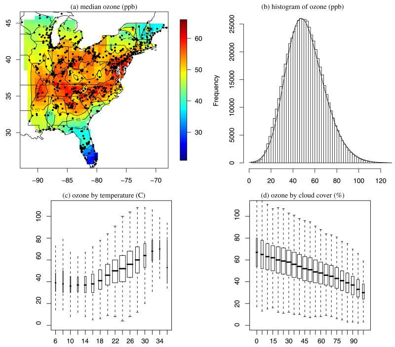
Figure 2.
Panel (a) maps the sample median ozone concentration; the points are the 631 monitoring locations. Panel (b) plots the skew-normal(34.5, 24.3, 1.8) over the histogram of ozone concentrations, pooled over spatial location. Panels (c) and (d) plot ozone by daily average temperature and cloud cover proportion, respectively; the data are pooled over space and the width of the boxplots are proportional to the number of observations in the bins. The online version of this figure is in color.

