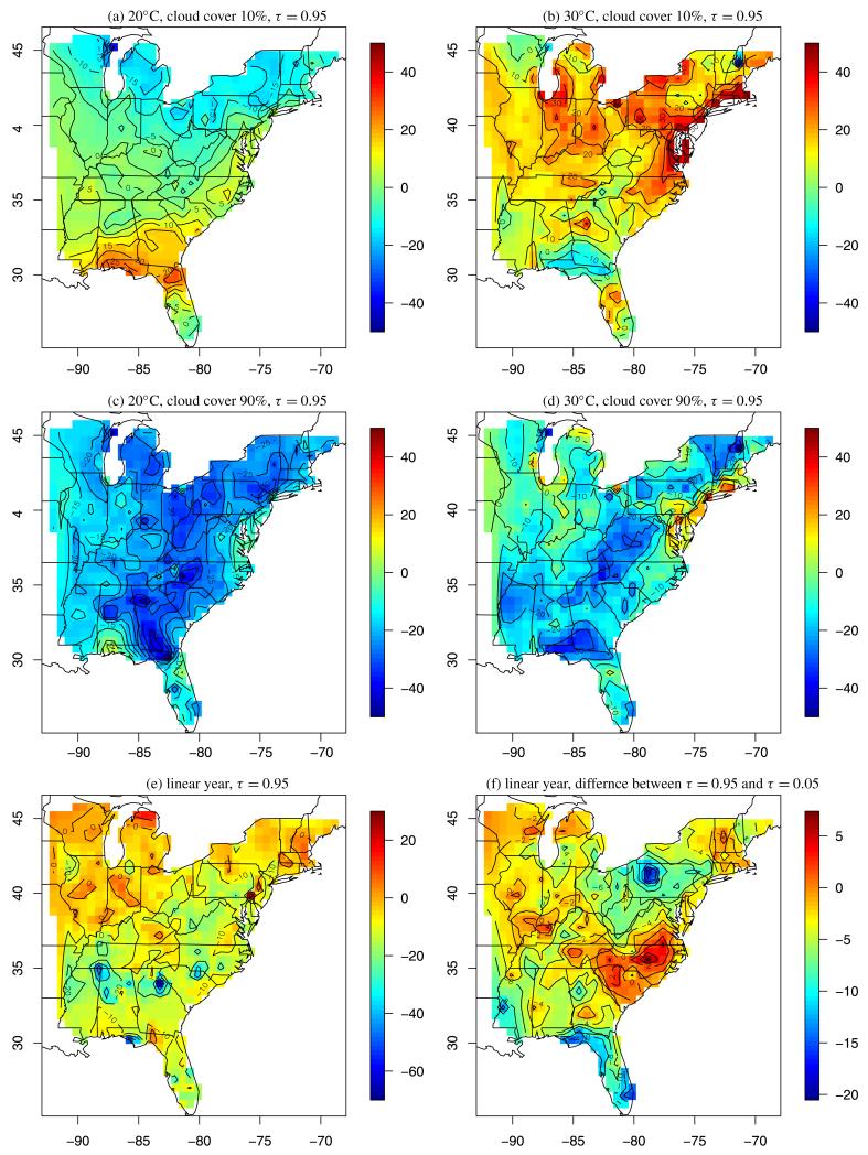
Figure 4.
Summary of the posterior mean of βj(τ, s). Panels (a)–(d) plot linear combinations of βj(τ, s) as discussed in (21). Panels (e) and (f) plot the posterior mean of βj(0.95, s) and βj(0.95, s) − βj(0.05, s), respectively. The units are parts per billion in all plots. The online version of this figure is in color.

