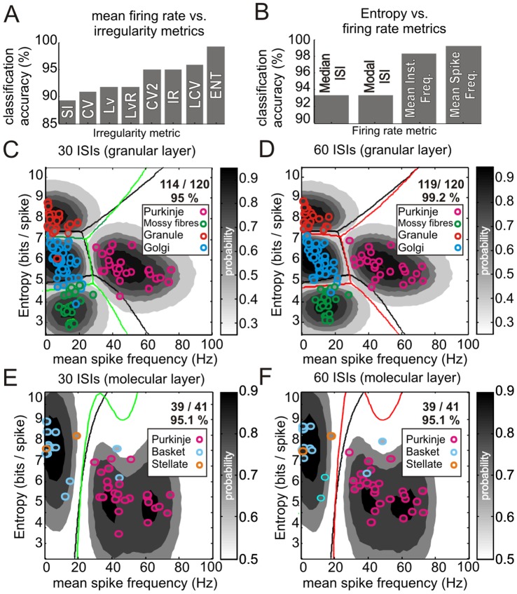
Figure 3. Comparison of irregularity measures, frequency measures and spike-train length on classification accuracy.

The bar chart shown in A plots the Gaussian Process Classifier LOO-CV accuracy for our rat dataset using a range of firing irregularity statistics combined with MSF. The worst combination was MSF vs SI offering 89% classification accuracy, whilst MSF vs. ENT performed at 99.2% accuracy. B shows a similar analysis with a variety of frequency measures combined with ENT. Median and Modal ISI offered ∼93% accuracy with a marginal difference between mean instantaneous frequency and mean firing rate (98% and 99.2%, respectively). C & D show Gaussian Process Classifiers built on the granular layer dataset but with 30 ISIs or 60 ISIs, respectively. The decision boundaries for the model built on all spikes are superimposed (black lines), along with the recomputed decision boundaries (green and red lines respectively). Note that the probability contours are specific to each model. Using 30 ISIs offered a prediction accuracy of 95% whilst the model built with 60 ISIs for all cells offered the same accuracy as the all-spikes model (99.2%; c.f. Figure 2H). This shows the model can be built and applied to spike trains containing as little as 60 ISI’s without a decrease in performance. This allows a prediction in the order of a few seconds for the slowest firing neurones (granule cells). E & F show Gaussian Process classifiers built on the molecular layer dataset following the same convention as above. Note that the probability contours are specific to each model. Using 30 or 60 ISIs offered prediction accuracy of 95.1% in both cases, comparable to the all-spikes model (92.7%; c.f. Figure 2P).