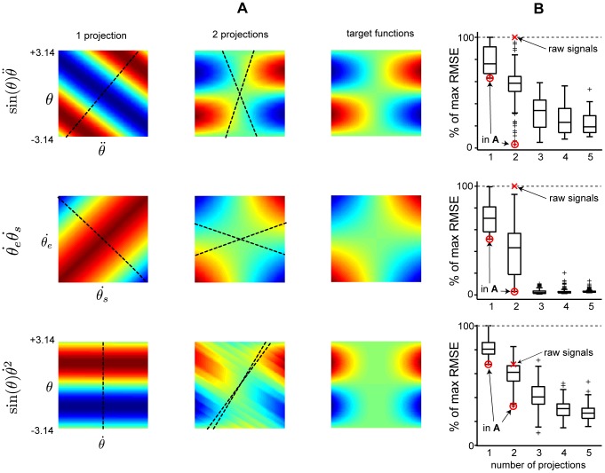
Figure 4. Approximation examples of basic non-linear functions.

(A) Approximated surfaces using a single or two projections (left and middle columns, respectively) compared to the approximated or target function surface (right-hand column) (i.e RMSE = 0). The colors represent the height of the surface ranging from negative values (blue) to positive values (red), comparable to the surface in Figure 2C. In each row, a different non-linear interaction retrieved from the terms within the inverse dynamics of the planar double joint arm in [79] is used. The illustrated projections had the lowest RMSE of 100 tested projections, each tested projection having a random direction. The actual RMSE values can be found in (B). The approximated surfaces also display the actual projections used as dashed lines above the surfaces. The value of the elbow angle variable, range between and , to capture an entire period of the sin function that is approximated. (B) RMSE of approximations of three two-dimensional non-linear terms in A. The approximations where constructed using random projection directions and a total of 60 GrCs. 100 approximations where constructed for each box. The mean RMSE is shown by the center line of the box, the boxes themselves extend to the 25th and 75th quartile and the whiskers extends to the most extreme RMSE not considered to be outliers, which are instead shown as black crosses. The red markers with an arrow from “raw signal” show the RMSE of approximations using the raw signals as projection directions, i.e. without recombination of inputs and those with an arrow from “in A” show the RMSE of the approximations shown in (A).