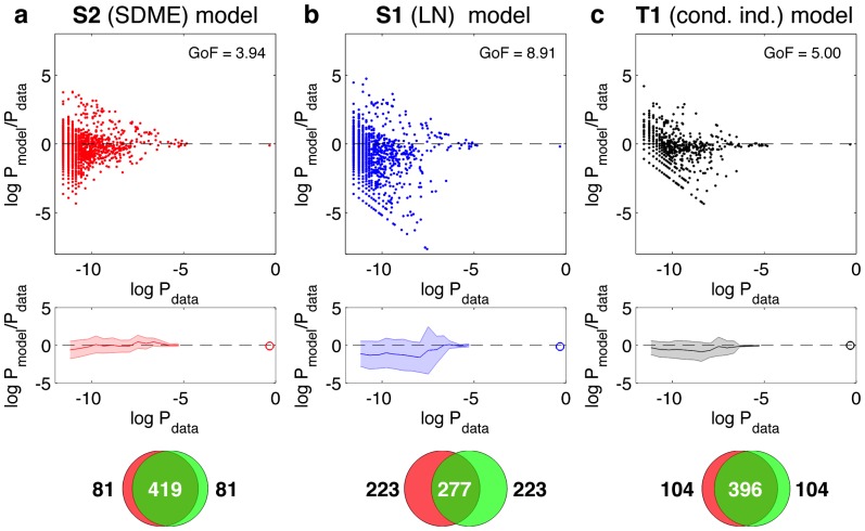
Figure 6. The performance of various models in accounting for the total vocabulary of the population,
 . The results for the S2 model are shown in (a), the results for the S1 model in (b), and the results for a full conditionally independent model (T1) in (c). The first row displays the log ratio of model to empirical probabilities for various codewords (dots), as a function of that codeword's empirical frequency in the recorded data. The model probabilities were estimated by generating Monte Carlo samples drawn from the corresponding model distributions; only patterns that were generated in the MC run as well as found in the recorded data are shown. GoF quantifies the deviation between true and predicted
  of the non-silent codewords shown in the plot; smaller values indicate better agreement (see Methods). The second row summarizes this scatterplot by binning codewords according to their frequency, and showing the average log probability ratio in the bin (solid line), as well as the
  std scatter across the codewords in the bin (shaded area). The highly probable all-silent state,
  , is shown separately as a circle. The third row shows the overlap between 500 most frequent patterns in the data and 500 most likely patterns generated by the model (see text). Models were fit on training repeats; comparisons are done only with test repeats data.

