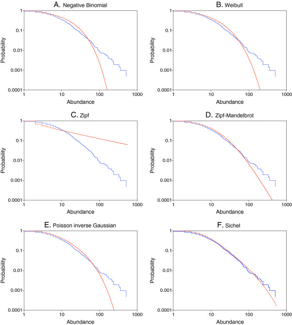
Figure 1.
Rank-frequency plots of protein abundances from the first experiment, together with fitted distributions.A. Negative binomial. B. Discrete Weibull. C. Zipf. D. Zipf-Mandelbrot. E. Poisson inverse Gaussian. F. Sichel. Observed data are depicted in blue, and the fitted distributions are depicted in red. As described in the Methods, we start with a listing of all the proteins, along with their frequency of occurrence (abundance). The complementary cumulative distribution P(x) of the abundance x is defined as the fraction of proteins with abundance greater than or equal to x. Our plots depict both the observed and the fitted complementary cumulative distributions (ordinates) vs protein abundances (abscissas).

