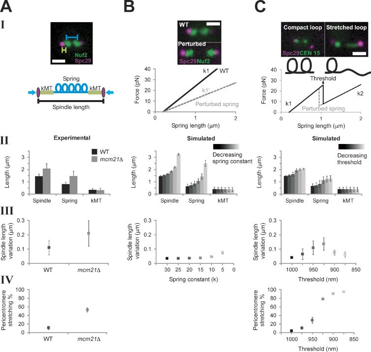
Figure 2.
Model simulations with a piecewise continuous spring recapitulate experimental observations. (A) Experimental data of WT and mcm21Δ cells (pericentromere depleted of cohesin). Spindle length (II) and pericentromere stretching (IV) were measured using population images of cells containing Spc29-RFP spindle poles and LacO at CEN15, respectively. Spindle length variation (III, fluctuation about the mean spindle length) was measured by tracking spindle poles over ∼10 min (Stephens et al., 2011). (B) Numerical simulations of spindle dynamics with a linear chromatin spring F = −k (Lspring − Lrest), in which Lrest = 200 nm (lighter = decreasing spring constant). The spring constant (k) was decreased to simulate perturbation of the spring (see B, I). Experimental images display an increase in the interkinetochore distance (distance between kinetochore clusters, Nuf2) in cohesin/condensin mutants. Simulations using a Hookean spring do not generate asymmetric pericentromere stretching. (C) Simulations of spindle dynamics with the spring defined by a piecewise continuous equation dependent on a threshold (lighter = decreasing threshold). (top) Experimental images reveal two spring states (compact, stretched) of a pericentromere LacO array. Under a force threshold (Lthreshold) the spring is looped (k1 and Lrest1, compact), and above the threshold, a loop stretches, adding length to the spring, which decreases the spring constant and increases the rest length (k2 and Lrest2, stretched). When Lspring < Lthreshold, F = −k1 (Lspring − Lrest). At Lspring ≥ Lthreshold, the spring constant is reduced from k1 to k2 (k2 = k1 (L1/L1 + Lopenloop)) and greater rest length (Lrest2 = Lrest1 + Lopenloop), giving F = −k2 (Lspring − Lrest2), in which the mean experimental aggregate spring length is L1 = 800 nm and Lopenloop = 450 nm (10 kb of nucleosomal chromatin from the stretched loop). (B and C) Simulated population measurements for linear (B) and nonlinear (C) spring models (spindle length [II] and pericentromere stretching [IV]) were generated by running the model and randomly selecting one time step [n = 500, five groups, 100 simulations each]). Simulated time lapses (III) were run for 1,000 s, 50 s for equilibrating, and 950 s measured (n = 25). Bars, 1 µm. Error bars represent standard deviation.

