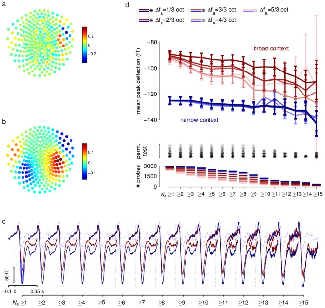
Figure 5. Local adaptation effects.

(a) Pattern of weights of the spatial filter used to extract the maximal signal-to-noise spatial projection of the MEG data. (b) The implied spatial pattern of the signal extracted by the filter shown in (a). (c) ERFs obtained by averaging responses to odd probes (solid lines) selected by threshold value of N_a (number of preceding tones falling outside a frequency window of width , here 1/3 octave). ERFs are separated by context (blue narrow; red broad). Shading for curves show regions averaged to obtain peak values in (d). Adaptation is evident for odd probes in the broad context but small or absent in the narrow context. ERFs for standard probes (dashed lines) are also shown for reference, and are not grouped by N_a. (d) Adaptation effects for a range of windows. Curves show ERF peaks (averaged as indicated in (c)) for odd probes in narrow (blue) and broad (red) context as a function of threshold value of N_a, calculated for different frequency exclusion windows (colour saturation, see legend at top). Error bars show standard errors. Grey stars indicate pairs of ERFs that were significantly different at the p<0.05 level according to a random permutation test. Lines at the bottom show the number of probe tones (combined across all subjects) that contribute to each ERF. Numbers fall as threshold N_a grows, contributing to greater uncertainty in measurements.