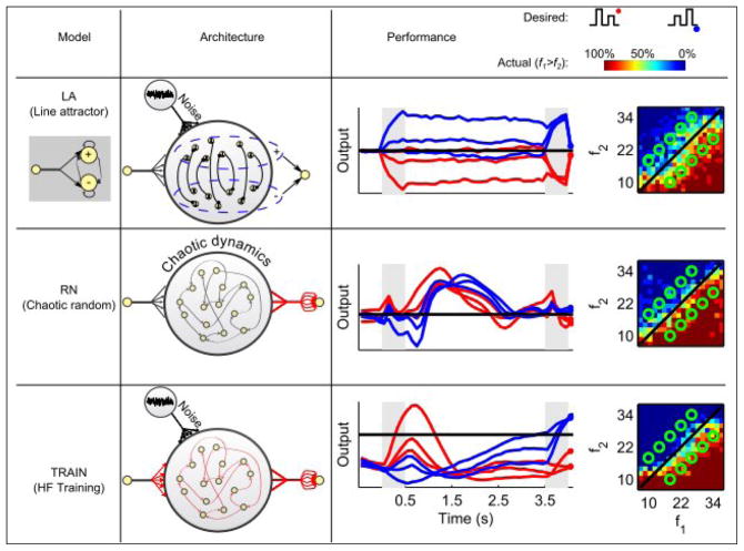
Figure 2. The three models.

Columns 1 and 2 illustrate the models we consider, column 3 shows the output of each model, and column 4 demonstrates model performance. Stimulus presentations times are indicated in gray in column 3, and the decision time is at the end of the time period shown. Red and blue traces correspond to f₁>f₂ and f₁<f₂, respectively, as indicated by the schematics above. Correct responses occur when the blue traces are positive and the red traces are negative at decision time. In column 4, performance is shown as the fraction of “f₁>f₂” responses for the entire f₁-f₂ plane (see colorbar above), with the 10 experimental frequency pairs indicated by the green circles. The LA model is composed of populations of spiking neurons (1^st column) receiving positive and negative tuned input during the stimulus (shaded) with self-excitation and mutual inhibition. The output is defined as the difference between the firing rates of the positive and negative populations. The RN model is composed of 1500 rate units randomly connected to each other, creating chaotic dynamics. 30% of the neurons receive external input during the stimuli, and the output is a trained linear readout from the entire network. The TRAIN model starts from a similar set up as the RN network, but all connections are trained (depicted in red) using the Hessian-Free algorithm. The output is a linear readout as for the RN model.