Figure 2.

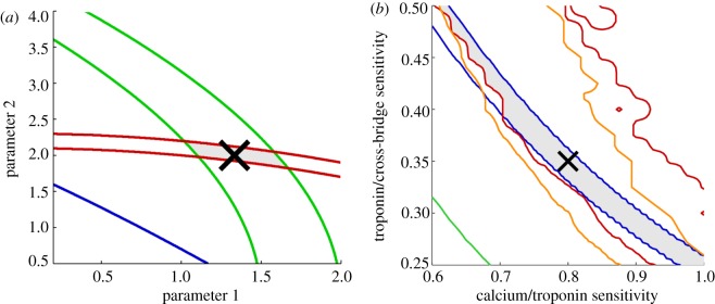
Visualization of model constraints. (a) A synthetic example. The two model parameters are constrained using three experimental constraints, visualized in green, red and blue. Each of the coloured lines represents the boundary of a region in which a specific experimental constraint is met, given variation in two parameters. The grey region represents the ‘viable region’ for the model parameters, which is the intersection of all the regions. This example visualization shows the green constraint as being most useful to refine experimentally, which would especially lead to a better estimate of parameter 1. The blue experimental constraint is too weak to be useful, being met in the vast majority of models, and would not be useful to refine, or include in fitting these model parameters. (b) Previous model results, for the sensitivity of troponin C binding to calcium (‘calcium/troponin sensitivity’) and the sensitivity of cross-bridge binding and tension generation to the fraction of bound troponin C (‘troponin/cross-bridge sensitivity’). In this particular case, the ‘blue’ constraint, related to the amount of tension generated, determines most of the constraint for both model parameters. The red and orange constraints also limit the region for parameter 2, although both parameters are still highly coupled. To indicate the relation of the final choice of parameters in the model to these constraints, this choice can be indicated in the visualization, such as by the ‘X’ in (b).