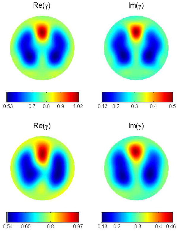
Figure 6.
Top row: Reconstruction from noise-free data for Example 3. The cut-off frequency was K = 5.2. The dynamic range is 71% for the conductivity, and 75% for the permittivity. Bottom row: Reconstruction from data with 0.01% added noise. The cut-off frequency was |k| ≤ 5.5. The dynamic range is 62% for the conductivity, and 68% for the permittivity.

