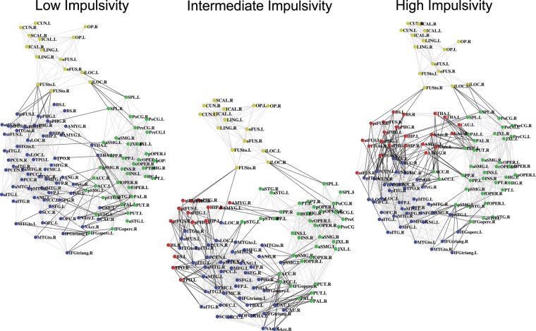
Figure 2.

Backbone plots visualizing the inter-regional FC for the low, intermediate, and high impulsivity groups. The connectivity backbone is derived in 2 steps (Hidalgo et al. 2007). First, we extracted within-module maximum spanning trees connecting all the nodes in each module such that connection weights are maximal. Secondly, connections across the whole network were added in order of their weight until a desired average node degree k (here, k = 14) was reached. The resulting connectivity backbone was then laid out in 2 dimensions using the Kamada–Kawai spring embedding algorithm (Kamada and Kawai 1989). Nodes are colored according to their module assignment: yellow = Module 1, green = Module 2, blue = Module 3, and red = Module 4. See Supplementary Table S4 for ROI abbreviations.