Figure 7.
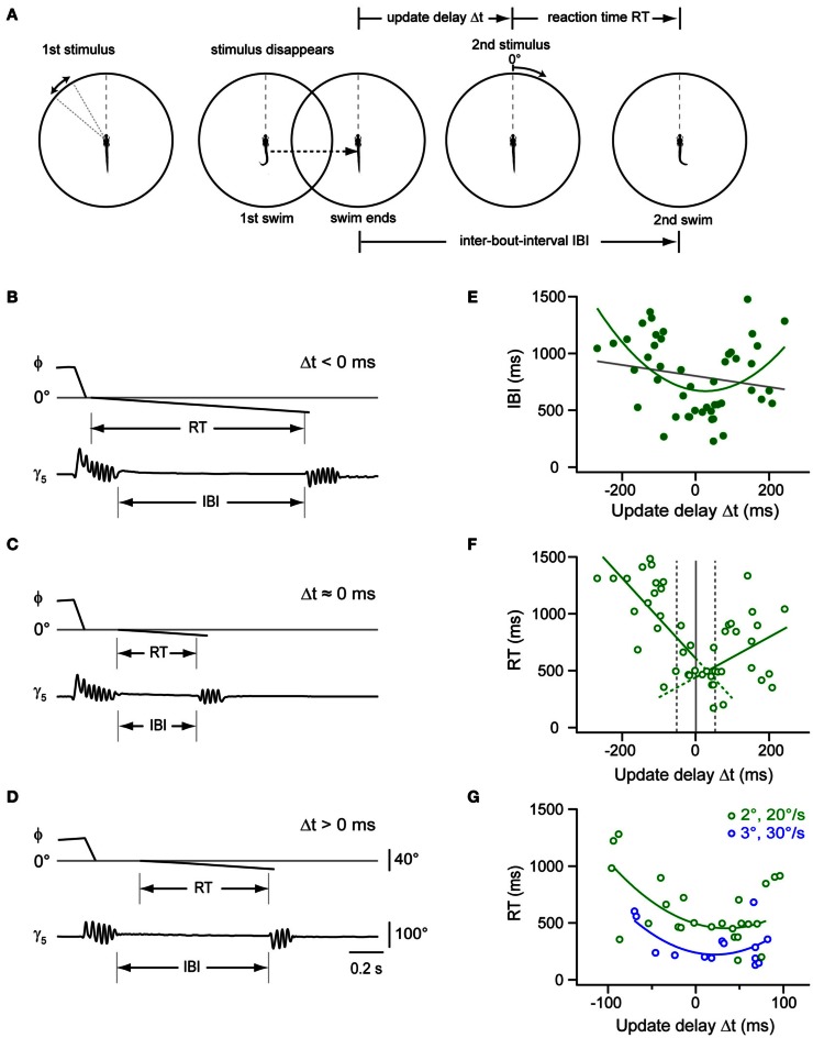
Impact of stimulus timing on inter-bout-intervals and reaction times in a two-step stimulus paradigm. (A) Schematic of a two-step stimulus paradigm with variable delay. First stimulus is a target moving in the periphery (35–55°; left panel), which eventually triggers a target-directed swim (second panel). Stimulus and background translate to center (0°), and the stimulus disappears. After a variable delay, the target reappears at the center and moves toward the periphery at constant size and speed (2°; 20°/s; 3rd panel), until the larva performs a second directed swim, which ends the trial (right panel). Update delays (Δt) and inter-bout-intervals (IBI) are measured relative to the end of the first swim, reaction time (RT) is measured from onset of second stimulus. (B) Time course of fish-target angle ϕ and caudal tail angle γ5 during paired swim bouts evoked by the two-step stimulus paradigm. The second stimulus appeared before the end of the first swim, corresponding to a Δt < 0 ms. Note long IBI. (C) Same as in (B), but with second stimulus appearing near end of first swim (Δt ≈0 ms). Note short IBI. (D) Same as in (B), but with second stimulus appearing after end of first swim (Δt > 0 ms). Note longer IBI. Scale bars apply to panel (B–D). (E) Scatter plot of IBIs vs. update delay (Δt). Gray line: straight line fit (rPearson = 0.18). Green curve: second order polynomial fit to the data (r = 0.46). Note minimum near Δt ≈ 0 ms (n = 47 trials from 13 fish). (F) Scatter plot of reaction times (RT) vs. update delays (Δt). Green lines: straight line fits to data points with negative and positive update delays (Δt), respectively (n = 47 trials from 13 fish). Broken gray lines represent three different delay groups i.e., Δt < -50 ms, -50 ms < Δt < 50ms, and Δt > 50 ms. (G) Scatter plot of RT values vs. update delays (Δt) on an expanded time scale (–100 to 100 ms). Reaction times are shorter when the second stimulus is larger and faster (3°; 30°/s; n = 14 trials from 5 fish; blue symbols) than under control conditions [2°; 20°/s; green symbols, same as in panel (F)]. Blue and green curves are second order polynomial fits to data points measured under the two conditions, respectively.

