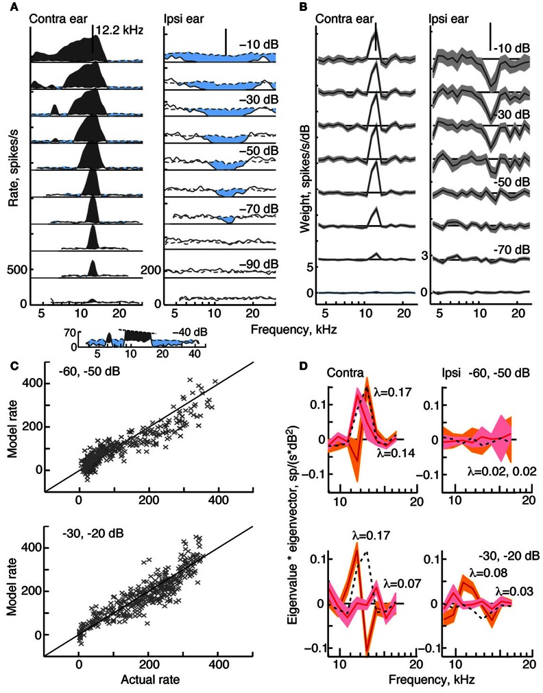
Figure 2.

Response characteristics for a type I neuron, BF 12.2 kHz. (A) Tone response maps showing rate responses to 200-ms tone bursts, plotted against the tone frequency at a fixed attenuation. Rates were computed from single tone presentations and smoothed (5-bin triangular filter) for display. Attenuations are shown at right. Zero dB attenuation was 94 dB SPL at the neuron's BF. Response maps were created by presenting tones in the contralateral ear only (left) and ipsilateral ear only (right). Discharge rates across the duration of the tone are shown by solid lines. Spontaneous rates are shown by dashed lines. The horizontal solid straight line indicates 0 spikes/s, and the rate scale is given at bottom left (different in the two ears). Excitatory responses are colored gray and inhibitory responses are light blue. The vertical lines at the top of the plots show the BF in the contralateral ear (12.2 kHz). (B) Weight functions estimated from responses to binaural RSS stimuli presented across a range of attenuations. First-order weights (w_C and w_I in Equation 1) are plotted on the same frequency axis as in (A). Weight estimates are shown as black lines, and gray regions indicate ±1 SEM. Contralateral and ipsilateral weight functions were derived from the same 200 responses to the binaural stimulus set. Note that the weight scales on the ordinate differ. (C) Rates predicted by the model (ordinate) vs. experimental rates (abscissa) in leave-one-out model testing. For each plot, data for two attenuations (indicated in the legend) were combined for the leave-one-out procedure. (D) Second-order effective filters (i. e., eigenvectors of M_C and M_I in Equation 3) for the same two fits shown in (C). Eigenvectors multiplied by their corresponding eigenvalue are plotted against frequency. The 1st-order weights, scaled to the same maximum value in each plot, are shown as black dotted lines. Only eigenvectors with the two largest positive eigenvalues λ are shown (largest λ, orange; second-largest λ, pink). The colored regions indicate ±1 SEM. The negative eigenvalues are smaller than the positive eigenvalues (<0.03, top case; <0.1, bottom case) and the corresponding eigenvectors are noisy (not shown).