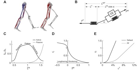
Fig. 2.

(A) A musculoskeletal model describing the geometry and force generation properties of 11 lower limb muscles used. (B) A Hill-type equilibrium model of muscle–tendon contraction dynamics. Muscle was represented as a passive elastic element in parallel with an active contractile element (CE). Tendon was represented as a non-linear elastic element in series with the muscle. The muscle–tendon length (L^MT) derived from the path geometry and joint angles was used to compute muscle fiber length (L^M), fiber shortening velocity (v^M), tendon length (L^T), pennation angle (α), muscle force (F^M) and tendon force (F^T). (C) The force–length curves modeled the effects, active/passive force–length multipliers f_AL and f_PL, of normalized fiber length, , on the active and passive force generated by muscle fibers. The active force–length curve included ascending, plateau and descending regions. (D) The force–velocity curve modeled the effect, force–velocity multiplier f_v, of normalized fiber velocity, , on the active force generated by muscle fibers. The force–velocity curve included shortening () and lengthening () regions. (E) The tendon force–strain curve modeled the proportion of maximum isometric force, tendon force–strain multiplier f_T, in the tendon as a function of the strain in the tendon []. The force in the tendon would equal maximum isometric force (i.e. f_T=1) at a tendon strain of 10% in the plantarflexors (PF) or 4% in all other muscles.