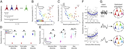
Fig. 4.

Populations optimized for stimulus representation combine homogeneity with diversity. (A) Cartoon of greedy search algorithm to estimate the population that best represents a particular type of stimulus. Neurons were iteratively added, one at a time, to the current population of neurons such that the neuron chosen maximized the population's reconstruction accuracy. To allow for homogeneity, neurons could be added more than once (e.g., two red neurons). (B and C) Visualization of the population selected to best represent a white-noise stimulus (B) or a low-frequency stimulus (C). Graphs show neurons (as dots) projected into a 2D space using principal component analysis (PCs). Population sizes vary from n = 1 to n = 10, numbers next to dots correspond to algorithm iteration step when each neuron was added. Note that certain neurons are chosen multiple times and that stimulus type dictates the selected population diversity. (D) GLM parameter diversity of the greedy-search-selected populations (blue) averaged over eight different choices of stimulus spectra relative to homogeneous (red) and randomly sampled heterogeneous populations (green), n = 10 neurons per population. Asterisks indicate where greedy search populations are significantly less diverse than heterogeneous (P < 0.05) and population diversity has been normalized to that of randomly sampled heterogeneous. Error bars indicate SEM (blue) and interquartile range (green). (E) Greedy-search population diversity for specific stimlus types. Colors indicate different stimulus types corresponding to inset power spectrum (magenta, stimulus as in B; cyan, Ornstein–Uhlenbeck process with τ = 10 ms; black, stimulus as in C), open circles indicate multiple runs of the greedy search algorithm (n = 10 per stimulus type), asterisks indicate significant differences in population diversity between stimulus types. (F) Population decoding error as a function of stimulus filter diversity for 200 randomly sampled populations (dots, n = 5 neurons per population) for stimulus 1 and 2 as in Fig. 3 (A and B, respectively). Least-squares fits using a second-order polynomial (blue) show that on average there is an intermediate level of stimulus filter diversity where decoding error is minimized (regression P < 0.01). (G) Cartoon showing that population diversity should be preferentially selected with respect to the specific incoming stimulus distribution.