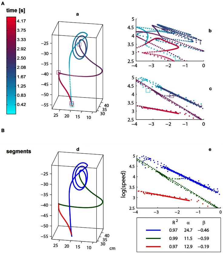
Figure 1.

The trajectories of an ISL “Cake” repetition before (a) and after (d) time-warping. (A) The samples of the raw data are colored according to time. (B) The time-warped trajectory, where the three colors designate power law segments. Log–Log plots of curvature and velocity are depicted on the right side: (b) raw data and (c,e) time-warping, colored according to time and segments, respectively. It can be seen that the spatial representation, i.e., path, of the raw and time-warped trajectories are identical. Also, although both raw and time-warped log–log curves are characterized by linear segments, the time warping is based on a simpler power law representation which is characterized by three highly fitting (R² > 0.97) segments with beta values ranging from about −0.19 to −0.6. The transitions between long straight segments in the log–log representation are made either by a very brief transitional period which does not comply with the power laws of the adjacent segments [e.g., the portion between the blue and green segments in (e)] or in the temporal point of intersection of the piecewise linear sections [e.g., green to red segment in (e)].