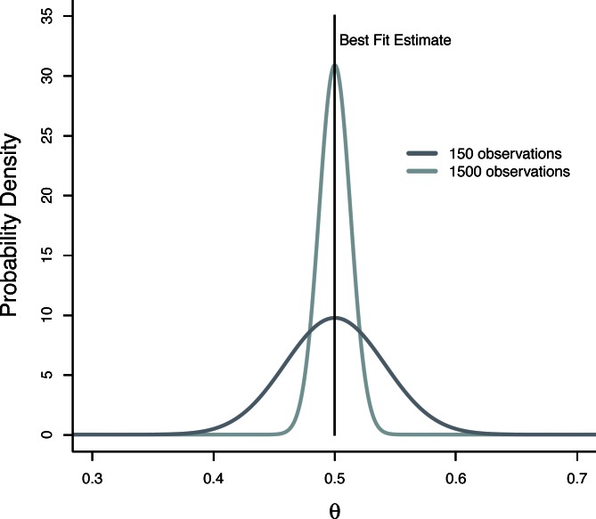
Figure 2.

Posterior probability distribution of θ. An example of the posterior probability of θ for hypothetical datasets. The vertical black line represents the optimal point estimate of θ that one would calculate by error minimization (the MLE). The other curves are the posterior probability distributions of θ for different sample sizes. Note that as the number of observations increases, the posterior distribution is narrowed as our confidence about the true value is improved. Also note that the maximum value of posterior probability coincides with the MLE that would be calculated by minimizing error. Calculating the posterior distribution over parameters provides not only an optimal point estimate, but also a quantification of parameter uncertainty.