FIGURE 4.

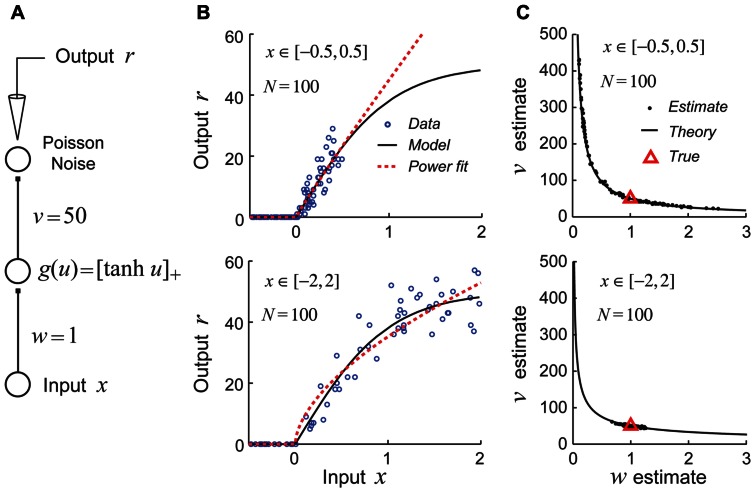
Example of continuous parameter confounding in a simple non-linear neural network model. Adapted with permission from DiMattina and Zhang (2010). (A) A simple three layer neural network whose input and output weight parameters (w,v) we wish to estimate from noisy stimulus–response data. Noise is drawn from a Poisson distribution. (B) Top: The input stimuli x ∈ [-0.5, 0.5] only drive the hidden unit over a limited region of its gain function (black curve) which may be well approximated by a power law function (red dashed line). Bottom: The input stimuli x ∈ [-2,2] drive the hidden unit over a larger region of its gain function which is poorly approximated by a power law function. (C) Top: When trained with sets of stimuli like that in the top of Figure 4B, the estimates (black dots) lie scattered along the curve predicted by the power law confounding theory. Bottom: When trained with sets of stimuli like those in the bottom panel of Figure 4B, the true parameter values (red triangle) are more reliably recovered.