Figure 2.

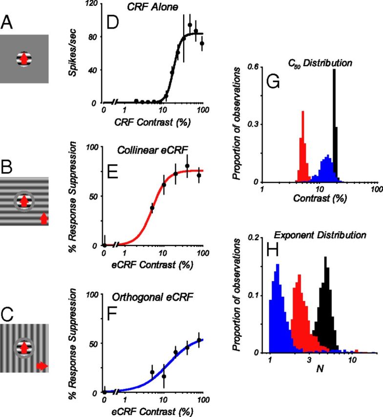
CRF and eCRF contrast response function comparison. A, Stimulus configuration for CRF alone, where a central patch of grating is optimized in orientation, spatiotemporal frequency, drift direction (red arrow), and size for the individual neuron. B, Stimulus configuration for CRF in the presence of a collinear eCRF, a central patch of grating as in A, simultaneously presented with a grating in the eCRF at the same spatiotemporal frequency and orientation. There was a small annular gray region that separated the center patch and the grating in the eCRF. The radius of the center patch was the optimal size for the CRF. The outer radius of the gray annulus was the size chosen from the expanding gray disk experiment where there was no response marked by the arrow in Figure 1C. C, Stimulus configuration for CRF in the presence of an eCRF stimulus oriented orthogonally to the central grating. For B and C, the gratings in the eCRF were presented at a range of contrasts, from 5 to 80%, in octave steps. D, The contrast response function for the CRF. E, Contrast-suppression function from the eCRF in response to collinear eCRF stimuli. F, Contrast-suppression function for orthogonal eCRF stimuli. D–F, The closed circles and error bars indicate mean ± 1 SD. Lines are best fits of the Naka–Rushton function to the data. For comparison of parameters between conditions, estimates of parameter distributions were achieved by repeated fitting to bootstrap samples of the data. G, Distributions of C₅₀. H, Distributions of exponent parameter, for CRF (black), collinear eCRF (red), and orthogonal eCRF (blue).