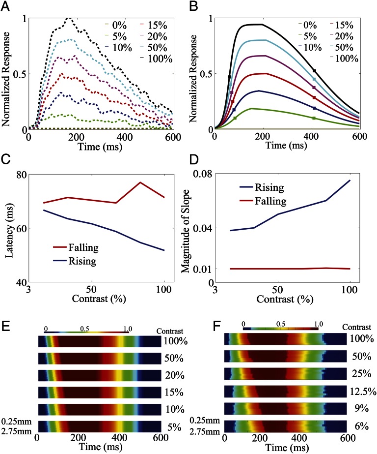
Fig. 2.

(A) Time course of the normalized responses to different contrasts in an annulus region in our MCN. (B) Logistic fits of the responses in A. Square symbols on each curve indicate the time when the response reaches half of the peak value in the rising and falling stages under each contrast, respectively. (C and D) Latencies (C) and slopes (D) in the rising (blue) and falling (red) stages for the fitted responses as a function of stimulus contrast. (E and F) Logistic fits of the time courses of the normalized responses at different locations for each stimulus contrast in our MCN (E) and in experiments (F) [adapted with permission from ref. 10 (Copyright 2009, Elsevier)]. A horizontal top row within each space-time subplot is closest to the center and the bottom row is farthest. Here, we follow the convention used in ref. 10 for the space–time plot under a given contrast that shows the fitted time course at one location within an annulus with inner radius 0.5 mm and outer radius 3.0 mm around the center of the 2D Gaussian fit.