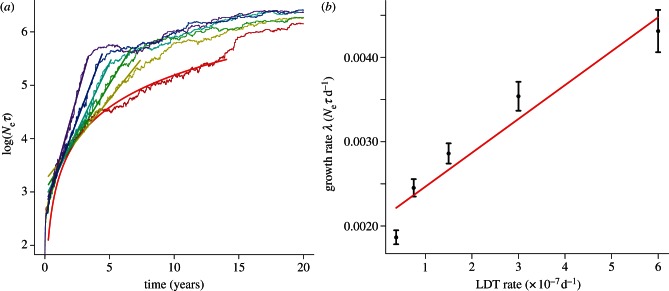
Figure 1.
(a) Skyline plots of the effective number of infections for six rates of LDT (red, ϕLDT = 0; yellow, ϕLDT = 3.73 × 10⁻⁸; green, ϕLDT = 7.5 × 10⁻⁸; cyan, ϕLDT = 1.5 × 10⁻⁷; blue, ϕLDT = 3 × 10⁻⁷; violet, ϕLDT = 6 × 10⁻⁷). Irregular curves show the mean of 40 replicate skyline plots for each rate of LDT. Smooth lines are the mean of 40 regressions fitted to 40 replicate skyline plots for each rate of LDT. The segmented regressions were fitted to the log-transformed effective number of infections (Neτ). For ϕLDT ≠ 0 we fit an exponential model to each of the 40 replicate skyline plots (e.g. Neτ = Ceλt), whereas for ϕLDT
= 0, we fitted a time-squared model (Neτ = π(vt + b)2). In each case, the mean regression is based on the mean of the parameters (e.g.  ). The regressions are based on Neτ during the spatial spread of infection. The beginning and ending times for spatial spread are parameters of the regression model and are estimated as part of the fit for each replicate skyline plot [53] (see the electronic supplementary material). (b) The change in the exponential rate of growth of the effective number of infections (Neτ) versus the rate of LDT (ϕLDT). Each point is the mean growth rate (λ) and the bars are the standard error of the mean. The red line is the linear regression fitted to the 240 growth rates computed from the model results (40 runs for each of five rates of LDT).

