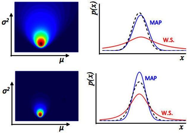
Figure 3.

Illustration of estimation uncertainty. These plots show the output of a numerical Bayesian estimation of the parameters of a Gaussian distribution. If x ~ (μ, σ²), and some values of x are observed, the likelihood of different values for μ, σ² can be calculated jointly using Bayes' rule. The colored plots (left) show the joint likelihood for different pairs of values μ, σ², where each point on the colored image is a possible pair of values μ, σ², and the color represents the likelihood of that pair of values. The line plots (Right panel) show the distribution across x implied by different values of μ, σ². The dashed black line is the true distribution from which data were drawn. The blue line is the maximum a-posteriori distribution—a Gaussian distribution with values of μ, σ² taken from the peak of the joint distribution over μ, σ² shown on the left. The red line represents a weighted sum (W.S.) of the Gaussian distributions represented by all possible values of μ, σ², weighted by their joint likelihood as shown in the figure to the left. The top represents an estimate of the environment based on fewer data points than the bottom row. With relatively few data points, there is a lot of uncertainty about the values of μ, σ², i.e., estimation uncertainty—illustrated by the broader distribution of likelihood over different possible values of μ, σ² (Left panel) in the top than bottom row. Whilst the maximum a-posteriori distribution is a good fit to the “true” distribution from which data were drawn in both cases, if we look at the weighted sum of all distributions, there is a lot more uncertainty for the top row case, based on fewer data points. Hence if the observer uses a weighted sum of all possible values of μ, σ² of the environment to calculate a probability distribution over x, the variance of that distribution depends on the level of estimation uncertainty.