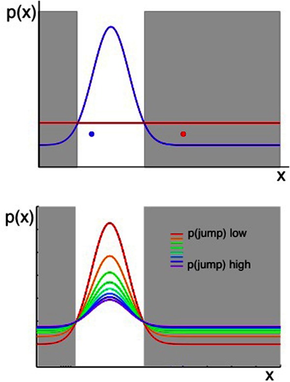
Figure 4.

Two considerations for evaluating whether a change has occurred. Plots show the probability of observing some value of x, given that x ~ (μ, σ²) and the values of μ, σ² can jump to new, unpredicted values as defined in Equation 2. When an observation of the environment is made, an algorithm that aims to determine whether a change has occurred should consider both the likelihood of the previous model of the environment given the new data, and the prior probability of change as determined in part by the transition function. Top panel: the probability of an observation taking a value x is shown in terms of two distributions. A Gaussian shown in blue represents the probability density across x if the most likely state of the environment (the most likely values of μ, σ²), given past data, were still in force. The uniform distribution in red represents the probability density across x arising from all the possible new states of the environment, if a change occurred. The possible new states are represented by a uniform function (red line in the figure) because, if we consider the probability of each value of x under an infinite number of possible states at once (i.e., the value of x given each of infinitely many other possible values of μ and σ²), the outcome is a uniform distribution over x. A change should be inferred if an observation occurs in the gray shaded regions—where the probability of x under the uniform (representing change) is higher than the probability under the prior Gaussian distribution. Hence the red data point in Figure 4 should cause the system to infer a change has occurred, whereas the blue data point should not. Bottom panel: as above, the probability distribution over x is a combination of a Gaussian and a Uniform distribution (representing the most likely parameters of the environment if there has been no change, and the possible new states of the environment if there has been a change, respectively). In this panel, the Gaussian and Uniform components are summed to give a single line representing the distribution over x. The different colored lines represent different prior probabilities of change, and hence different relative weightings of the Gaussian and uniform components. Increasing the prior probability of change results in a wider distribution of probability density across all possible values of x.