Statistical geometry of lattice chain polymers with voids of defined shapes: Sampling with strong constraints

Abstract

Proteins contain many voids, which are unfilled spaces enclosed in the interior. A few of them have shapes compatible to ligands and substrates, and are important for protein functions. An important general question is how the need for maintaining functional voids is influenced by, and affects other aspects of proteins structures and properties (e.g., protein folding stability, kinetic accessibility, and evolution selection pressure). In this paper, we exam in detail the effects of maintaining voids of different shapes and sizes using two-dimensional lattice models. We study the propensity for conformations to form a void of specific shape, which is related to the entropic cost of void maintenance. We also study the location that voids of a specific shape and size tend to form, and the influence of compactness on the formation of such voids. As enumeration is infeasible for long chain polymer, a key development in this work is the design of a novel sequential Monte Carlo strategy for generating large number of sample conformations under very constraining restrictions. Our method is validated by comparing results obtained from sampling and from enumeration for short polymer chains. We succeeded in accurate estimation of entropic cost of void maintenance, with and without an increasing number of restrictive conditions, such as loops forming the wall of void with fixed length, with additionally fixed starting position in the sequence. Additionally, we have identified the key structural properties of voids that are important in determining the entropic cost of void formation. We have further developed a parametric models to predict quantitatively void entropy. Our model is highly effective, and these results indicate that voids representing functional sites can be used as an improved model for studying the evolution of protein functions, and how protein function relates to protein stability.

I. INTRODUCTION

Proteins are the working molecules of cell. Understanding how they maintain their stability and carry out their functions is a fundamental problem of molecular biology. Although it is well-known that the structures of proteins are well packed^1–3, there exist numerous packing defects in the form of voids buried in the interior of proteins. The size distributions of these voids are broad⁴. Various scaling relationships indicate that their origin may be generic steric constraints of compact chain polymers^4,5. It is also well-known that a few voids on a protein may play key roles in enabling protein functions^6–9, for example, for substrate and ligand binding.

However, the shape space of voids of folded and unfolded proteins are not well-characterized, and the energetic consequences and the kinetic effects by maintaining voids of certain shape and size are largely unknown. In this paper, we exam in detail the effects of maintaining voids of different shapes in lattice models of chain polymers. Lattice models have been widely used for studying protein folding, where the conformational space of simplified polymers can be examined in detail^10–18. Despite its simplistic nature, lattice model has provided important insights about proteins, including collapse and folding transitions^16,19–23, influence of packing on secondary structure and void formation^11,12,24,25, the evolution of protein function^26,27, nascent chain folding¹⁸, and the effects of chirality and side chains²⁵.

In this paper, we focus on conformations that enclose voids of specific shapes. Our main objective is to study the fraction of conformations with a specific void shape among all possible conformations. This is related to the entropic cost of maintaining such a void in a polymer structure. We also study the location that voids of a specific shape and size tend to form, and the influence of compactness on the formation of such voids. The methodology we use is the sequential Monte Carlo approach (SMC) designed for sampling conformations under strong constraints, i.e., the requirement of the existence of specific types of voids. SMC is a growth-based method, in which residues are added to the chain polymer one by one until the conformation of full length is obtained. This method is first used in reference²⁸ to estimate the average extension of molecular chains. The basic goal is to obtain a set of conformational samples, along with the probabilities of generating these conformations. Compared with other sampling methods, such as Markov chain Monte Carlo^29–31, sequential Monte Carlo can generate diverse samples and can directly estimate the number of conformations containing voids of specific shapes accurately. In this study, we develop several new strategies to improve the effectiveness of sequential Monte Carlo in generating samples under strongly constrained conditions.

Our paper is organized as follows. In section 2, we describe briefly the lattice model and define void and shape of voids. We then discuss the constrained sequential Monte Carlo method used in our study. Results are presented in Section 3. The final section contains the summary and conclusion.

II. METHOD

A. Lattice Model

In lattice models, chain polymers are self-avoiding walks (SAWs) in the square lattice space ℤ². A length n conformation is denoted by a connected chain X_n = (x₁, x₂, ⋯, x_n), where the i-th monomer is located at the site x_i = (a_i, b_i), where a_i and b_i are integers. The Manhattan distance between bonded monomers x_i and x_i+1 is 1. The chain is self-avoiding: x_i ≠ x_j for all i ≠ j. We consider the beginning and the end of a polymer to be distinct. Only conformations that are not related by translation, rotation, and reflection are considered to be distinct. This is achieved by following the rule that a chain is always grown from the origin, the first step is always to the right, and the chain always goes up at the first time it deviates from the x-axis. We denote the set of all length-n SAW polymers satisfying these constraints as 𝒫_n.

B. Voids and shape of voids

Given the conformation X_n ∈ 𝒫_n of a chain polymer, the unoccupied sites on the square lattice are divided by the polymer into disconnected components:

$${\mathbb{Z}}^2\backslash X_n=u\cup {\upsilon }_1\cdots \cup {\upsilon }_k,$$

where u is the outside component that connects to infinity, and υ₁, ⋯, υ_k are the voids that are enclosed by X_n. Here two components are considered connected if they share any edges or vertices. By this definition, conformations (a) and (b) in Figure 1 both have a size-2 void, but conformation (c) does not contain any void, since the internal two unoccupied points are connected to the outside through a vertex. This definition of void is arbitrary, but is consistent with the definition of contact for monomers in a chain, that is, only if two sites in a void shares an edge, they are considered to be connected²⁴.

Fig 1.

Conformations in square lattice model. (a) This conformation contains a size-2 void. (b) This conformation contains a size-2 void. (c) This conformation does not contain any void.

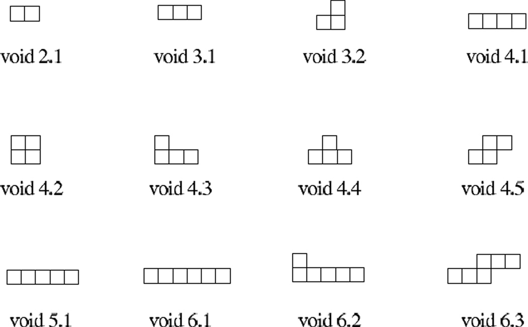
We are interested in the set of conformations with voids of a particular shape S. Figure 2 shows some of those shapes of sizes 2 to 6. Note that those shapes are regular shapes, in which sites are connected by edges. In this study we do not consider shapes with sites connected by a vertex only, such as the size-2 void formed by conformation (b) in Figure 1. Here the voids are labelled by their shapes, where the first digit represents the number of sites the void occupies, and the second digit is the identification number of different shapes.

Fig 2.

Regular shapes of voids of different sizes. Here the first digit represents the number of sites the void occupies, and the second digit is the identification number for different shapes. All possible shapes for voids up to size 4 are listed. Several samples for voids of size 5 and 6 are also listed.

C. Parameters of interest

To study the properties of conformations with specific shaped, we consider the following parameters.

a. Propensity of void formation f₁(S, n)

Let Ω_n(S) be the set of conformations with at least one void of a specific shape S, that is

$${\mathrm{\Omega }}_n(S)=\{X_n|X_n\in {𝒫}_n,X_n\text{ has at least one void of shape }S\}.$$

The fraction of conformations with void of this particular shape S among all possible conformations is:

$$f_1(S,n)=\frac{N(S,n)}{N_{\mathit{\text{all}}}(n)}=\frac{{\displaystyle {\sum }_{X_n\in {\mathrm{\Omega }}_n(S)}}1}{{\displaystyle {\sum }_{X_n\in {𝒫}_n}}1}.$$ (1)

This parameter represents the propensity of void formation, i.e., the probability of forming a void of specified shape. This relates to the question whether there are preferred shapes for binding voids to occur.

b. Propensity of void formation with fixed loop length f₂(l, S, n)

The loop length of a void is defined as l = I₁ − I₀ + 1, where I₀ and I₁ are the smallest and largest indices of the monomers forming the boundary of the void. Let Ω_n(l, S) ⊂ Ω_n(S) be the set of length n conformations with at least one void of shape S of loop length l. The fraction of conformations with void of a particular shape S and a particular void loop length l among all conformations with a void of the same shape but without the restriction of void loop length is defined as:

$$f_2(l,S,n)=\frac{N(l,S,n)}{N(S,n)}=\frac{{\displaystyle {\sum }_{X_n\in {\mathrm{\Omega }}_n(l,S)}}\xi (X_n,l,S)/K(X_n,S)}{{\displaystyle {\sum }_{X_n\in {\mathrm{\Omega }}_n(S)}}1},$$ (2)

where K(X_n, S) is the number of shape-S voids in X_n, ξ(X_n, l, S) is the number of shape-S voids with loop length l in X_n. This special treatment on N(l, S, n) is to deal with the cases when X_n has multiple voids of shape-S. In such cases, X_n is counted once in N(S, n), and counted 1/K(X_n, S) in N(l, S, n) for each combination of shape-S void and loop length l. For example, if conformation X_n has two voids of shape S, then K(X_n, S) = 2. If both voids have loop length l = 14, then ξ(X_n, l = 14, S) = 2 and this conformation contributes 1 to N(l = 14, S, n); if one void has loop length l = 14 and the other void has loop length l = 16, then this conformation contributes 1/2 to N(l = 14, S, n) and 1/2 to N(l = 16, S, n). Clearly, with this definition, we have

$${\displaystyle \sum _l}N(l,S,n)=N(S,n).$$

The parameter f₂(l, s, n) represents the propensity of void formation with fixed loop length, i.e., the probability of forming a void of specified shape with fixed void loop length. In protein, a related interesting question is how easier it is to form certain types of voids in shape and size with more local compared to with more global sequence fragments.

c. Propensity of void formation with fixed loop length and starting position f₃(I₀, l, S, n)

Let Ω_n(I₀, l, S) ⊂ Ω_n(l, S) be the set of length n conformations with at least one void of shape S, loop length l, and starting at residue position I₀. The fraction of conformations with void of a particular shape S, a particular loop length l, and a particular starting residue I₀ among the conformations with a void of the same shape and the same loop length^12,32 is defined as

$$f_3(I_0,l,S,n)=\frac{N(I_0,l,S,n)}{N(l,S,n)}=\frac{{\displaystyle {\sum }_{X_n\in {\mathrm{\Omega }}_n(I_0,l,S)}}\xi (X_n,I_0,l,S)/K(X_n,S)}{{\displaystyle {\sum }_{X_n\in {\mathrm{\Omega }}_n(l,S)}}\xi (X_n,l,S)/K(X_n,S)},$$ (3)

where ξ(X_n, I₀, l, S) is the number of shape-S voids with loop length l and starting residue I₀ in X_n. Similarly, this definition ensures that

$${\displaystyle \sum _{I_0}}N(I_0,l,S,n)=N(l,S,n).$$

The parameter f₃(I₀, I, S, n) represents the propensity of void formation with fixed loop length and starting position, i.e., the probability of forming a void of specified shape with fixed void loop length starting at a specific position. A related question in protein is what is the propensity of forming voids of certain shape with more local or more global sequence fragments starting at specific positions of the chain.

d. Propensity of void formation at specific compactness f₄(ρ, S, n)

The compactness of a polymer ρ is defined as t/t_max(n)¹¹, where t is the number of contacts in the conformation, and t_max(n) is maximum number of contacts possible for length n conformations. For square lattice space, we have¹¹:

$$t_{\text{max}}(n)=\{\begin{array}{cc}n-2b,\hfill & \text{if }{b}^2<n\le b(b+1),\hfill \\ n-2b-1,\hfill & \text{if }b(b+1)<n\le {(b+1)}^2,\hfill \end{array}$$

where b is a positive integer. Let Ω_n(ρ) ⊂ 𝒫_n be the set of length n conformations with compactness ρ and Ω_n(ρ, S) ⊂ Ω_n(ρ) be the set of length n conformations with at least one void of shape S and compactness ρ. The fraction of conformations of a particular compactness ρ with void of a particular shape S among all conformations with the same compactness ρ is defined as:

$$f_4(\rho ,S,n)=\frac{N(\rho ,S,n)}{N(\rho ,n)}=\frac{{\displaystyle {\sum }_{X_n\in {\mathrm{\Omega }}_n(\rho ,S)}}1}{{\displaystyle {\sum }_{X_n\in {\mathrm{\Omega }}_n(\rho )}}1}.$$ (4)

This parameter represents the propensity of void formation with certain compactness, i.e., the probability of forming a void of specified shape for length n chain polymers at a fixed compactness.

D. Estimating void parameters using sequential Monte Carlo

Exhaustive enumeration can be used to calculate the propensities defined above, but is only applicable to very short polymer chains. For longer chain, we use a modified version of the sequential Monte Carlo (SMC) method.

All the parameters described above are fractions, where the corresponding numerators and denominators N(S, n), N(l, S, n), N(I₀, l, S, n) and N(ρ, S, n) can be written in the form of

$${\displaystyle \sum _{X_n\in {\mathrm{\Omega }}_n(S)}}h(X_n),$$ (5)

where h(·) is a function of conformation X_n. Specifically, we have:

$$-h(X_n)=1\text{ for }N(S,n);$$

$$-h(X_n)={𝕀}_{{\mathrm{\Omega }}_n(l,S)}(X_n)\frac{\xi (X_n,l,S)}{K(X_n,S)}\text{ for }N(l,S,n);$$

$$-h(X_n)={𝕀}_{{\mathrm{\Omega }}_n(I_0,l,S)}(X_n)\frac{\xi (X_n,I_0,l,S)}{K(X_n,S)}\text{ for }N(I_0,l,S,n);$$

$$-h(X_n)={𝕀}_{{\mathrm{\Omega }}_n(\rho ,S)}(X_n)\text{ for }N(\rho ,S,n),$$

where 𝕀_Ωn(X_n) is the indicator function, 𝕀_Ω(X_n) = 1 if X_n is in set Ω_n, 𝕀_Ω(X_n) = 0 otherwise.

Suppose we can generate random samples of conformations $X_n^{(j)}$, j = 1, ⋯, m, from a trial distribution g(X_n). Following the importance sampling principle^33,34, formula (5) can be estimated as:

$$\frac{1}{m}{\displaystyle \sum _{j=1}^m}\frac{h(X_n^{(j)}){𝕀}_{{\mathrm{\Omega }}_n(S)}(X_n^{(j)})}{g(X_n^{(j)})}\approx {𝔼}_g[\frac{h(X)·{𝕀}_{{\mathrm{\Omega }}_n(S)}(X_n)}{g(X)}]={\displaystyle \sum _{X\in {\mathrm{\Omega }}_n(S)}}\frac{h(X)}{g(X)}·g(X)={\displaystyle \sum _{X_n\in {\mathrm{\Omega }}_n(S)}}h(X_n),$$ (6)

Note that to obtain an unbiased estimate, the trial distribution g(X_n) must have a support larger than h(X_n)𝕀_Ωn(S)(X_n), that is, g(X_n) > 0 must hold for all X_n in Ω_n(S) that satisfy h(X_n) > 0. Let $w_n^{(j)}=1/g(X_n^{(j)})$ to be the weight of sample $X_n^{(j)}$, then Eqn (6) can be rewritten as

$${\displaystyle \sum _{X_n\in {\mathrm{\Omega }}_n(S)}}h(X_n)=\frac{1}{m}{\displaystyle \sum _{j=1}^m}{w}_n^{(j)}h(X_n^{(j)}){𝕀}_{{\mathrm{\Omega }}_n(S)}(X_n^{(j)}).$$ (7)

The efficiency of the estimator of Eqn (6) depends on the choice of the trial distribution g(X_n) and the computational complexity for generating a sample. In general, if g(X_n) is approximately proportional to |h(X_n)𝕀_Ωn(S)(X_n)|, with a support larger but close to Ω_n(S), the estimate can be reasonably accurate³⁴.

The original Rosenbluth and Rosenbluth growth method generates samples in the space of 𝒫_n ²⁸. Starting at x₁ = (0, 0), monomers are added to the chain and the associated weights are updated recursively, until the chain reaches length n. Modifications of the algorithm can be found in^24,34–36. However, the space under our consideration is a highly constrained subspace of 𝒫_n. For example, for void shape 4.1 and chain length 50, the size of the constrained space Ω_n(S) is less than 2 × 10⁻³ of the size of 𝒫_n. With additional constraints such as fixed loop length, the space becomes even smaller and sampling such conformations becomes more difficult. The simple growth method of²⁸ is very inefficient in generating samples for such constrained space. Below we reformulate the sampling space and modify the growth method to overcome this difficulty.

1. An equivalent representation of Ω_n(S)

In order to avoid location ambiguity, the construction of 𝒫_n is restricted to the set of SAW conformations starting at x₁ = (0, 0), x₂ = (1, 0) and going up at the first time the chain deviates from the x-axis. Since our main interests are sampling conformations containing specific void, we adopt an equivalent representation that is more efficient for our purpose.

Specifically, let υ = υ(S) be a set of sites in ℤ², whose union takes the shape S. Let A(υ) = (a₁(υ), ⋯, a_|A(υ)|(υ)) be the set of neighboring sites of υ, sharing either edges or vertices with υ. We call it the wall sites of υ. If a SAW completely occupies A(υ) and does not intersect with υ, then this SAW has at least one void of shape S. Denote the set of all such conformations as

$$G_n(\upsilon )=\{X_n|X_n\text{ is a SAW},A(\upsilon )\subset X_n,\upsilon \cap X_n=\varnothing \}.$$

Recall that by definition a conformations in 𝒫_n first grows to the right, and always goes up when it first deviates from the x-axis. Note that the conformations in G_n(υ) is not restricted to 𝒫_n as they can start from any site on the lattice. In G_n(υ), we consider two SAWs as equivalent if one SAW can be transformed into the other through a combination of rotation, reflection and position translation. Then G_n(υ) consists of a number of disjoint equivalent classes.

It can be easily established that there is a one-to-one mapping between conformations in Ω_n(S) and the equivalent classes of conformations in G_n (υ) through transformation consisting the primitives of rotation, reflection, and translation. Each of the transformations provides such a map that the starting site x₁ of X_n ∈ G_n(υ) becomes the origin (0, 0), the second site x₂ becomes (1, 0), and the first site that deviates from x-axis is up. Hence, if h(·) is a function of X_n that takes the same value for equivalent conformations, we have:

$${\displaystyle \sum _{X_n\in {\mathrm{\Omega }}_n(S)}}h(X_n)={\displaystyle \sum _{X_n\in G_n(\upsilon )}}\frac{h(X_n)}{E(X_n,S)}.$$

where E(X_n, S) is the number of equivalent conformations of X_n in G_n(υ).

The number E(X_n, S) depends on K(X_n, S), the number of shape-S voids contained in X_n (as in Eqn (2)), and the symmetricity of the shape-S. Let q(υ) be the number of combination of rotation and reflection that maps υ to itself. In two-dimensional lattice space, there are 4 possible rotations and 2 possible reflections around x and y axes. Hence, q(υ) can only take a value in {1, 2, 4, 8}. For example, q(υ) = 8 for shape 4.2 in Figure 2, q(υ) = 4 for shapes 2.1 and 3.1, q(υ) = 2 for shapes 4.4 and 4.5, and q(υ) = 1 for shape 4.3.

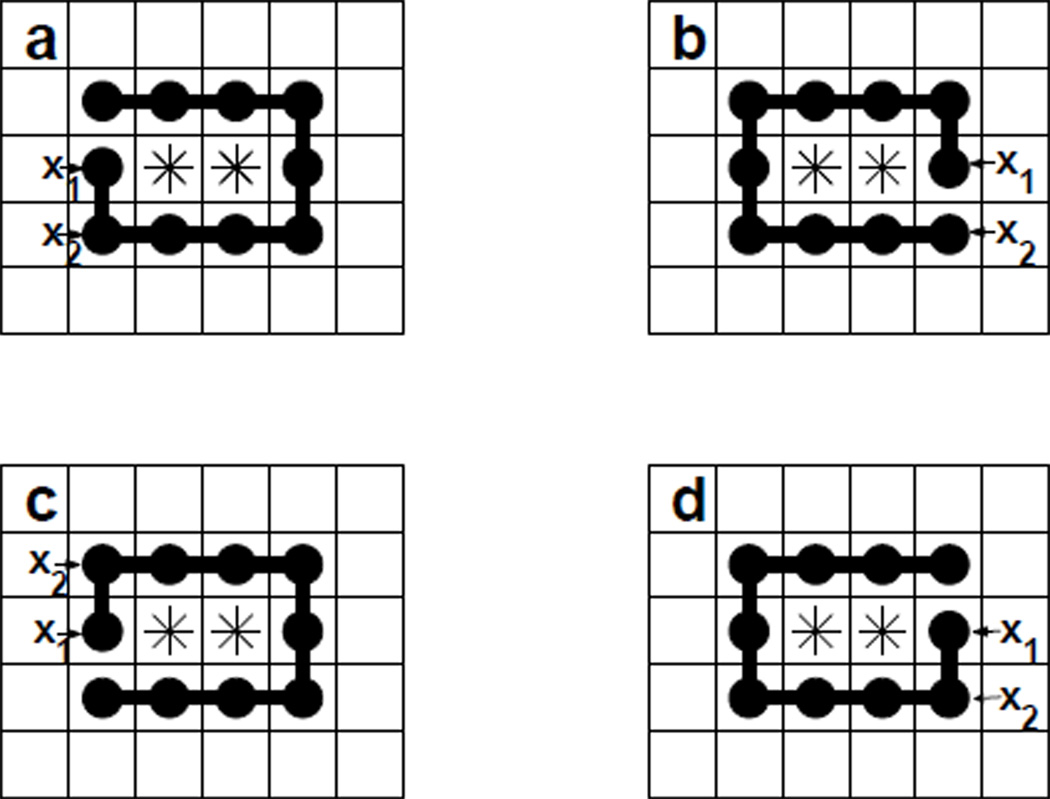
When X_n contains only one S-shaped void, the size of its equivalent class E(X_n, S) is q(υ). Figure 3 shows 4 polymers in a equivalent class for void 2.1. When X_n contains total K(X_n, S) S-shaped voids, then E(X_n, S) = q(υ)K(X_n, S) as each of the voids contributes q(υ) number of members in the equivalent class.

Fig 3.

The equivalent class of conformations. The union of the sites occupied by stars (*) is the fixed void υ. Here polymer a, b, c and d are different chains enclosing void υ, as indicated by the different sites occupied by the starting monomer x₁ and the next monomer x₂. However, the shapes of the polymers taken up by the union of the occupied sites for these chains are the same. As a consequence, these four polymers are equivalent.

Fig 4.

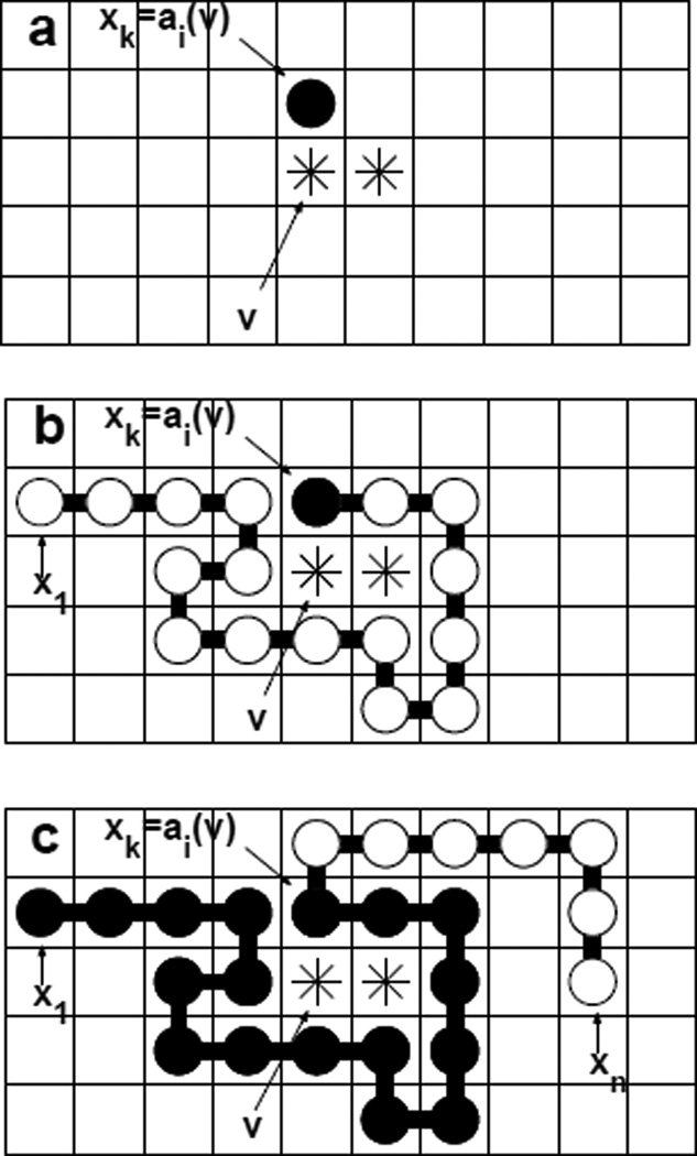
The general procedure for growing chains. The union of the sites occupied by stars (*) is the fixed void υ. (a) The k-th monomer y₁ = x_k is first placed to the position a_i(υ) of the wall sites of the void υ. (b) We then grow backward until we reach the first monomer y_k = x₁ of the chain to form void υ. (c) We continue by growing forward until we reach X_n.

To simplify our analysis, we note that G_n(υ) consists of disjoint subsets:

$$G_n(\upsilon )={\displaystyle \underset{i,k}{\cup }}{G}_n(\upsilon ,i,k),$$

where

$$G_n(\upsilon ,i,k)=\{X_n|X_n\in G_n(\upsilon ),x_k=a_i,A(\upsilon )\subset \{x_1,\dots ,x_k\}\}.$$

If X_n ∈ G(υ, i, k), then the void υ is completely enclosed by the prefix (x₁, ⋯, x_k) of the chain, where x_k is the last monomer in the prefix and occupies the i-th site a_i(υ) of the wall sites. We have k ≥ |A(υ)| since some of the monomers in the prefix (x₁, ⋯, x_k) may not be on the wall of the void. The remaining chain, (x_k+1, …, x_n), does not intersect with the void space υ nor with the wall sites A(υ).

Using this partition, we have that for any function h(·) that is constant within the equivalent classes,

$${\displaystyle \sum _{X_n\in {\mathrm{\Omega }}_n(S)}}h(X_n)={\displaystyle \sum _{X_n\in G_n(\upsilon )}}\frac{h(X_n)}{q(\upsilon )K(X_n,S)}=\frac{1}{q(\upsilon )}{\displaystyle \sum _{i,k}}{\displaystyle \sum _{X_n\in G_n(\upsilon ,i,k)}}\frac{h(X_n)}{K(X_n,S)}.$$ (8)

In the following we develop procedures to estimate the quantity

$${\displaystyle \sum _{X_n\in G_n(\upsilon ,i,k)}}\frac{h(X_n)}{K(X_n,S)},$$

for each subset G_n(υ, i, k), i = 1, ⋯, |A(υ)|, k = |A(υ)|, ⋯, n.

2. Algorithmic steps

The following procedure is used to generate Monte Carlo samples in G_n(υ, i, k) for all υ, i and k, which are then used to estimate the parameters listed in Section 2.3. First, we set x_k = a_i(υ) as defined by G_n(υ, i, k). We then grow backwards sequentially to place x_k−1, x_k−2, ⋯, until we reach the first monomer x₁ of the chain. During this process, the wall sites A(υ) become fully occupied by monomers in {x₁, …, x_k}, and the void space υ remains unoccupied. Lastly, as now that (x₁, ⋯, x_k) are placed and the constraints for void formation are satisfied, we complete the remaining conformation by sequentially placing monomers x_k+1, ⋯, X_n. The only constraint at this stage is that these monomers avoid the partial chain grown so far. An illustration of the procedure is shown in Figure 4.

For ease of presentation, we rearrange the monomer labels based on the above procedure. Define y_n = (y₁, …, y_n) as (x_k, …, x₁, x_k+1, …, x_n). Formally, y_s = x_k−s+1 for s ≤ k, and y_s = x_s for s > k. In this notation, the chain prefix of length s becomes y_s = (y₁, …, y_s).

We adopt the general framework of optimal sampling method³⁷ to generate sample conformations. Let m_i be the number of samples we retain in the i-th iteration, and m_max be the maximum value of {m_i}. In the initial step, we set m₁ = 1, $y_1^{(1)}=a_i(\upsilon ),\text{and }{w}_1^{(1)}=m_{\text{max}}$. For s = 2, …, n, we perform the following procedure:

1. At step s when adding the s-th monomer, assume there are m_s−1 samples $\{{\mathit{y}}_{s-1}^{(j)},j=1,\cdots ,m_{s-1}\}$ with weights $w_{s-1}^{(j)}$.

2. We now add the s-th monomer to the partial chain y_s−1. For each sample ${\mathit{y}}_{s-1}^{(j)}$, j = 1, ⋯, m_s−1, generate $l_s^{(j)}$ number of new samples ${\mathit{ỹ}}_s^{(j)}$ by placing y_s at each of the vacant sites neighboring $y_{s-1}^{(j)}$, where $l_s^{(j)}$ is the number of vacant sites neighboring $y_{s-1}^{(j)}$ in sample ${\mathit{y}}_{s-1}^{(j)}$. Set weight ${\mathrm{w̃}}_s^{(l)}=w_{s-1}^{(j)}$. Assume this step results in a total of $L_s={\displaystyle {\sum }_j}{l}_s^{(j)}\text{ samples }({\mathit{ỹ}}_s^{(l)},{\mathrm{w̃}}_s^{(l)})$.

   Note that the step k + 1 is slightly different. At steps 1, …, k, we grow the chain backwards. But at step k + 1, we start to grow the chain forward. That is, we place y_k+1 = x_k+1, which is connected to y₁ = x_k. Hence, at the step k + 1, we consider the vacant neighbor(s) of y₁, not y_k.

3. Assign a priority score ${\beta }_s^{(l)}$ to each resulting partial chain ${\mathit{ỹ}}_s^{(j)}$. The choice of the priority scores will be discussed in details in the next section.

4. If L_s < m_max, we keep all of the samples with their weights, set m_s = L_s and go to step s + 1. If L_s > m_max, we choose m distinct samples from $\{{\mathit{ỹ}}_s^{(l)},l=1,\cdots ,L_s\}$ according to the priority scores as follows:

   1. Find a constant c such that ${\displaystyle {\sum }_{l=1}^{L_s}}\text{min}\{c{\beta }_s^{(l)},1\}=m_{\text{max}}$.
   2. Choose distinct integers J₁, J₂, ⋯, J_mmax from l = 1, ⋯, L_s, with probability $b_s^{(l)}\equiv \text{min}\{c{\beta }_s^{(l)},1\}$. This is achieved by the following steps:

      1. Draw a sample r₀ from the uniform distribution between 0 and 1. Let r_j = j − r₀ for j = 1, ⋯, m_max;
      2. For each j = 1, ⋯, m_max, choose J_j as the integer such that ${\displaystyle {\sum }_{l=1}^{J_j-1}}{b}_s^{(l)}<r_j\le {\displaystyle {\sum }_{l=1}^{J_j}}{b}_s^{(l)}$ holds.
   3. Let ${\mathit{y}}_s^{(j)}={\mathit{ỹ}}_s^{(J_j)}$ and update its weight to be $w_s^{(j)}={\mathrm{w̃}}_s^{(J_j)}/\text{min}\{c{\beta }_s^{(J_j)},1\}$.

3. Priority scores

The priority score guides the growth of conformations, and its design is critically important for obtaining accurate estimates. Our priority scoring function has three components addressing three important issues, namely, the support of the target distribution, the weighting scheme of samples, and the look-ahead strategy.

The support of the target distribution

If a partial chain ${\mathit{ỹ}}_s^{(l)}$ at step s is impossible to eventually grow into the constrained space G_n(υ, i, k) at step n, it should be removed from future steps of sampling immediately at step s, since it is destined to be rejected. Define the support 𝒮_s of partial chains of length s as

$${𝒮}_s=\{{\mathit{y}}_s|\mathrm{s}.\mathrm{t}.\exists {\mathit{y}}_{s+1:n}=(y_{s+1},\dots ,y_n)\text{ that }({\mathit{y}}_s,{\mathit{y}}_{s+1:n})\in G_n(\upsilon ,i,k)\}$$

That is, 𝒮_s contains all possible prefix chains of length s of desired polymers. However, it is difficult to evaluate if a partial chain is in the support. Here we use a sequence of the support ψ_s that contains 𝒮_s but easy to work with. Specifically, let ψ₁ = {a_i(υ)} where the chain starts according to the definition of G_n(υ, i, k). The support ψ_s is updated sequentially as follows: For each partial chain y_s−1 ∈ ψ_s−1, find all possible chains y_s by adding a monomer to a vacant neighboring site which shares an edge with y_s−1. The new support ψ_s is the union of all such chains satisfying the following conditions:

1. y_s ∩ y_s−1 = ∅ (the self-avoiding constraint) and y_s ∉ υ, where υ is the void space.

2. If s ≤ k and if A(υ) \ y_s is not an empty set (i.e., the wall sites has not been filled by y_s), then A(υ) \ y_s must remain as a strongly connected set. Here we define that a strong connection exists between two sites if they share an edge.

3. If s ≤ k and if A(υ) \ y_s ≠ ∅, then the site y_s must satisfy

   $$k-s\ge d(y_s,A(\upsilon )\backslash {\mathit{y}}_s)+|A(\upsilon )\backslash {\mathit{y}}_s|-1,$$

   where d(y_s, A(υ) \ y_s) is the minimum Manhattan distance between y_s and the unoccupied wall sites, |A(υ) \ y_s| is the number of unoccupied wall sites of A(υ) \ y_s.

Condition (ii) reflects the property that both the filled and unfilled sites on the wall of the void must remain strongly connected at any time of the growth. Otherwise, the unfilled wall sites A(υ) has multiple not strongly connected components. In such cases, the self-avoiding property must be violated in order to fill all of them by y_n ∈ G_n(υ, i, k). This is the consequence of the Jordan curve theorem in plane³⁸.

Condition (iii) is to ensure that the remaining chain length is sufficient to fill all wall sites, i.e., A(υ) \ y_s must be filled by (y_{s + 1}, …, y_k), which is a length k − s chain connected to y_s. The priority scores without lookahead. In the optimal sampling method framework (³⁷), the priority score serves both as the propagation trial distribution as well as the resampling priority score. Under the importance sampling principle³⁴, the ideal trial distribution should be proportional to |h(x)π(x)|, where π(x) is the target distribution. In our case, it translates to ${\mathrm{w̃}}_t^{(l)}h({\mathit{ỹ}}_t^{(l)}){𝕀}_{{\psi }_t}({\mathit{ỹ}}_t^{(l)})$. Here $h({\mathit{ỹ}}_t^{(l)})$ is the value of function h(·) applied to partial chain ${\mathit{ỹ}}_t^{(l)}$, which is always non-negative.

For s > k, we simply set equally priority scores ${\beta }_s^{(l)}\equiv 1.0$ to all partial chain samples ${\mathit{ỹ}}_s^{(l)}$, since this stage is relatively easy.

For the more difficult part of the growth s ≤ k where the major constraints lie, we need to guide samples to grow into the support region ψ_s in order to reduce the sample rejection rate. Following Zhang and Liu³⁶, we use the priority score to achieve this. Taking condition (iii) when updating the support into consideration, we define

$$U_s({\mathit{ỹ}}_s^{(l)},\upsilon )=\{\begin{array}{cc}k-s+2-d({ỹ}_s^{(l)},A(\upsilon )\backslash {\mathit{ỹ}}_s^{(l)})-|A(\upsilon )\backslash {\mathit{ỹ}}_t^{(l)}|,\hfill & |A(\upsilon )\backslash {\mathit{ỹ}}_t^{(l)}|>0,\hfill \\ 0,\hfill & |A(\upsilon )\backslash {\mathit{ỹ}}_t^{(l)}|=0.\hfill \end{array}$$

It evaluates how much freedom and flexibility the remaining chain possess. When $|A(\upsilon )\backslash {\mathit{ỹ}}_t^{(l)}|>0$, there are still some vacant sites on the void wall needs to be occupied. In this case, if $U_s({\mathit{ỹ}}_s^{(l)},\upsilon )\le 0,{\mathit{ỹ}}_s^{(l)}$ is not in the support ψ_s, as it violates condition (iii), we reject this sample. The larger $U_s({\mathit{ỹ}}_s^{(l)},\upsilon )$ is, the less constrained the remaining chain is.

Combining the value of the function $h({\mathit{ỹ}}_t^{(l)})$ to be evaluated, and $U_s({\mathit{ỹ}}_s^{(l)},\upsilon )$ reflecting the desired flexibility of the remaining chain, we design our priority score for s ≤ k as:

$${\beta }_s^{(l)}={\mathrm{w̃}}_s^{(l)}h({\mathit{ỹ}}_s^{(l)}){𝕀}_{{\psi }_s}({\mathit{ỹ}}_s^{(l)})\text{ exp}\{-U_s^{-\frac{1}{2}}({\mathit{ỹ}}_s^{(l)},\upsilon )/T_s\},$$

where T_s is a temperature-like variable. The choice of values for T_s is important. In general, the constraint of forming void is not of serious concerns at the beginning, so we can use high values of T_s to enhance diversity in sampling. As the chain grows, the concern of meeting the constraints become stronger, since there are less freedom for the remaining chains to grow. Hence, we gradually reduced the T_s, as in simulated annealing algorithms. In this study, we use $T_s=\sqrt{k-s+16}$ for s = 1, ⋯, k − 1.

Priority score with look-ahead

An often used strategy to improve performance of SMC is look-ahead^36,39,40. Look-ahead enables us to use information from possible future steps to construct priority scores, resulting smaller rejection rate of the samples. In addition, it reduces the variance of samples for estimation and hence improves sample efficiency⁴¹.

For a δ-step look-ahead, the priority score at time t is determined by exploring all possible combinations of δ-step growth from the current sample y_s. Specifically, the priority scores we use are:

$${\beta }_s^{(l)}={\mathrm{w̃}}_s^{(l)}{\displaystyle \sum _{y_{s+1},\cdots ,y_{s+\delta }}}h({\mathit{ỹ}}_{s+\delta }^{(l)}){𝕀}_{{\psi }_{s+\delta }}({\mathit{ỹ}}_{s+\delta }^{(l)})\text{ exp}\{-\frac{U_s^{-\frac{1}{2}}({\mathit{ỹ}}_{s+\delta }^{(l)},\upsilon )}{T_s}\}$$

where ỹ_s+δ denotes (ỹ_s, y_s+1, ⋯, y_s+δ).

Note that as look-ahead step δ increases, the effectiveness increases at the cost of exponentially growing computational complexity. Hence the choice δ is a tradeoff between estimate efficiency and complexity. In this study we use δ = 1.

4. Estimation

In our framework, it is possible to estimate the parameters described in Section IIC for polymer chains of different lengths up to n when generating conformation samples of length n.

Specifically, when generating conformation samples for G_n(i, k), at step s = k, k + 1, ⋯, n, the generated partial conformations are ${\mathit{ỹ}}_s^{(l)}=(x_1^{(l)},\cdots ,x_k^{(l)},\cdots ,x_s^{(l)})$, which are properly weighted chain polymers of length s. Hence, ${\displaystyle {\sum }_{{\mathit{x}}_{n^{*}}\in G_{n^{*}}(\upsilon ,i,k)}}\frac{h({\mathit{x}}_{n^{*}})}{K({\mathit{x}}_{n^{*}},S)}$, n* = k, k + 1, ⋯, n, can be estimated by the following estimator

$$ĥ({\mathit{x}}_{n^{*}};i,k)=\frac{1}{m_{\text{max}}}{\displaystyle \sum _{l=1}^{L_s}}{\mathrm{w̃}}_s^{(l)}\frac{{𝕀}_{G_{n^{*}}(\upsilon ,i,k)}({\mathit{ỹ}}_s^{(l)})h({\mathit{ỹ}}_s^{(l)})}{K({\mathit{ỹ}}_s^{(l)},S)}$$

at step s = n*. Here the estimation is made after step (2) of the algorithmic steps in the previous subsection.

After generating samples for G_n(i, k) of all possible i, k, for any n* ≤ n, we can estimate ∑_{Xn* ∈Ωn*(S)} h(X_n*) by

$${\displaystyle \sum _{X_{n^{*}}\in {\mathrm{\Omega }}_{n^{*}}(S)}}h(X_{n^{*}})\approx \frac{1}{q(\upsilon )}{\displaystyle \sum _{i,k}}ĥ({\mathit{x}}_{n^{*}};i,k)$$

according to Eqn (8).

III. RESULTS

In this section, we present the results of estimation of the parameters described in Section 2.3. We also develop parametric models relating to void and chain properties for interpreting the estimated results, and for prediction of propensity of forming void of specific shape.

A. Propensity of void formation

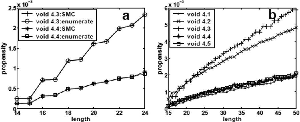
For propensity of void formation f₁(S, n) defined in Eqn (1), we first examine size-4 voids. There are 5 different shapes for size-4 regular voids (Figure 2). To validate our procedure, the estimated propensity of void formation is compared with the true values obtained by exhaustive enumeration, for chains of length 14 to 24. Figure 5(a) shows the results for voids shapes 4.3 and 4.4. The estimated values are indistinguishable from the true values. These results suggest that our sampling method works well and can provide accurate estimations.

Fig 5.

Estimating void propensity values. (a) Estimated propensity values and true propensity values of forming size-4 voids of different specific shapes for conformations of length 14 − 24. They superimpose very well. (b) Estimated propensity values of forming size-4 voids of different specific shapes for conformations of length 15 − 50.

The results for longer chains of length 15 to 50 using the SMC procedure are presented in Figure 5(b), where propensity of void formation f₁(S, n) for void shapes 4.1 to 4.5 are shown. It is clear that voids of different shapes have significant difference in propensity of formation. This raises the question whether voids and binding sites in proteins are similarly biased, and whether the distribution of voids of different shapes can be partly explained by these intrinsic propensities analogous what is observed here on lattice models.

a. Predictive models

To better understand our estimation results and to infer general principles, we develop a predictive model for f₁(S, n) using the following parametric form:

$$\widehat{f_1}(S,n)=\frac{1}{q(\upsilon )}{c}_1{c}_2^{-|A(\upsilon )|}{(n-|A(\upsilon )|+1)}^{c_3}[1-c_4(|e(\upsilon )|-4)],$$ (9)

where q(υ) represents the degeneracy of the void shape as we discussed in Section IID1. We consider three factors other than q(υ) in our model: the the wall size |A(υ)|, the chain length n, and number of outer corners of void, |e(υ)|. Here the outer corners, e(υ), are defined as the sites on void wall that connect to the void through a single vertex only. The values of q(υ), |A(υ)|, and |e(υ)| for different void shapes are summarized in Table I.

TABLE I.

Geometric features of voids determining the fractions of chain polymers containing such voids. q(υ) is related to the symmetry of the void υ, |A(υ)| is wall size of the void υ, and |e(υ)| is the number of outer corners of void υ.

void type	2.1	3.1	3.2	4.1	4.2	4.3	4.4	4.5	5.1	6.1	6.2	6.3
q(υ)	4	4	2	4	8	1	2	2	4	4	1	2
|A(υ)|	10	12	12	14	12	14	14	14	16	18	18	18
|e(υ)|	4	4	5	4	4	5	6	6	4	4	5	6

In this model, c₁, c₂, c₃, c₄ are positive constants. As the wall size |A(υ)| increases, it is expected that the propensity of forming voids of the specific shape decreases exponentially. This is reflected by the term containing $c_2^{-|A(\upsilon )|}$. When the chain length n increases, it is expected that the propensity of forming voids of the specific shape increases by some power. This is captured by the term of (n − |A(υ)| + 1)^c₃. We also find that the number of outer corners, |e(υ)|, is an important determinant of propensity of void formation. For void shapes with more outer corners, chain polymers enclosing such voids have more concave turns on the wall. This makes it more difficult for a self-avoiding chain to enclose the void. The negative term of |e(υ)| in Eqn (9) models this effect.

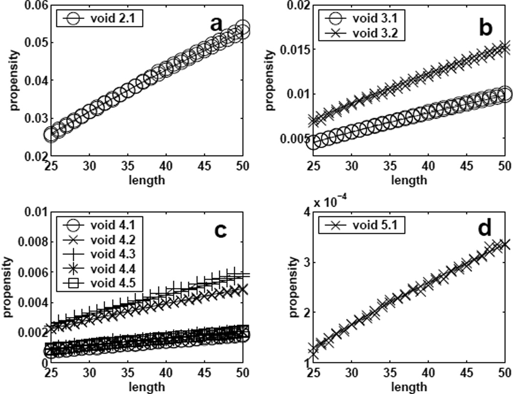
We estimate the coefficients in model (9) using the estimated f₁(υ_n) from SMC for voids of sizes 2 to 5 and chain length from 25 to 50. Taking log transformation and using nonlinear regression, we found that ĉ₁ = 47.46, ĉ₂ = 2.28, ĉ₃ = 0.76 and ĉ₄ = 0.21.

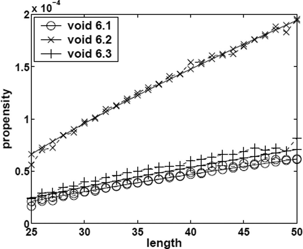
The propensity values estimated from SMC and the fitted results of $\widehat{f_1}(S,n)$ using model (9) are plotted in Figure 6. It can be seen that the parametric model fits the data very well. Using the above estimated parameters obtained from the training data, we develop a predictive model for the propensity for void shapes 6.1, 6.2 and 6.3, which are not used in deriving the regression model. The predictions are again compared with those estimated by SMC (Figure 7). The models works well, although it consistently under-estimates by a small amount for void shape 6.3.

Fig 6.

Propensity values of forming voids (size=2 – 5, a–d) of different specific shapes for conformations of length 25–50. These are used to develop a regression model. Dashed line: results obtained by estimation using sequential Monte Carlo. Solid line: fitted results from the regression models.

Fig 7.

Estimated and predicted propensity values of forming size-6 voids of different specific shapes for conformations of length 25 – 50. Dashed line: SMC results. Solid line: predicted results using the regression model (9).

B. Propensity of void formation with fixed loop length

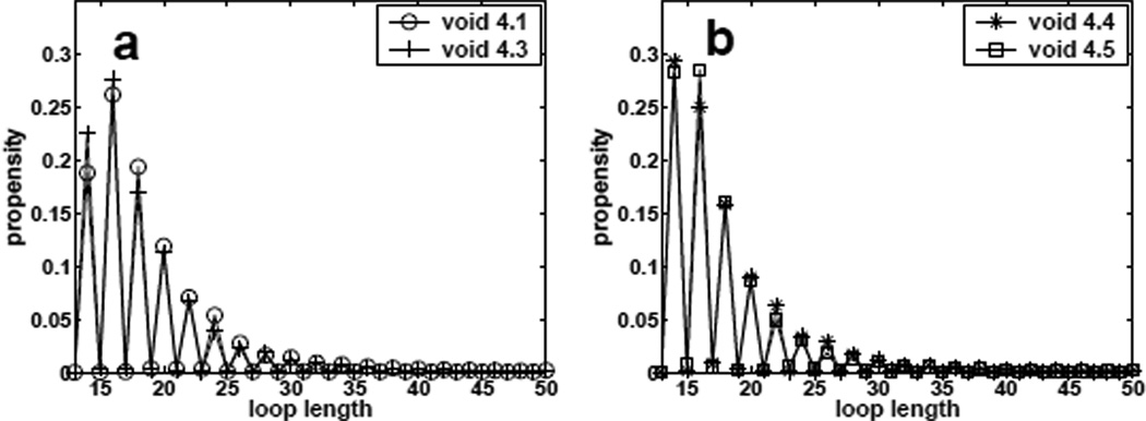
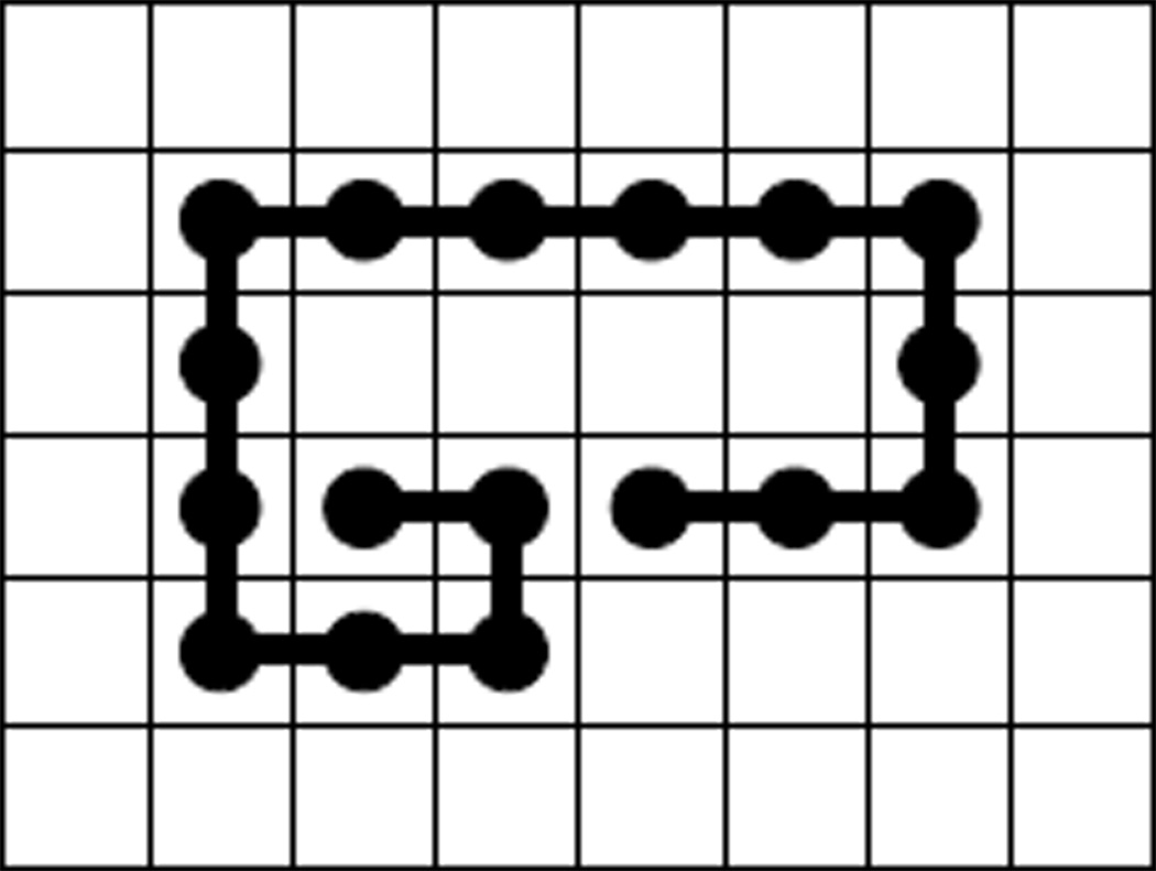
Now we consider the propensity of void formation with fixed loop length f₂(S, n) defined in Eqn (2). We plot estimated f₂(l, S, n = 50) for different specified loop length l and shape S in Figure 9. Although void with odd loop length do exist, we can see that it is much easier to form void with even loop length. This is because the number of wall sites, |A(υ)|, is always an even number on lattice. To form a void υ with odd loop length, the first monomer and the last monomer of the polymer on the void wall A(υ) cannot be adjacent, which results in a more complicated shape. A conformation enclosing a void of shape 4.1 with loop length 17 is given in Figure 8. On average, void shapes 4.1 and 4.3 have larger loop sizes than void shapes 4.4 and 4.5, because they have fewer corners. These results suggest that voids of different shapes have different propensity at specific loop lengths.

Fig 9.

Estimated propensity values of forming size-4 voids of different specific shapes with different specified loop length for conformations of length n = 50.

Fig 8.

Conformation with odd loop length. This conformation encloses an void of shape 4.1 with loop length 17.

C. End effect for void formation

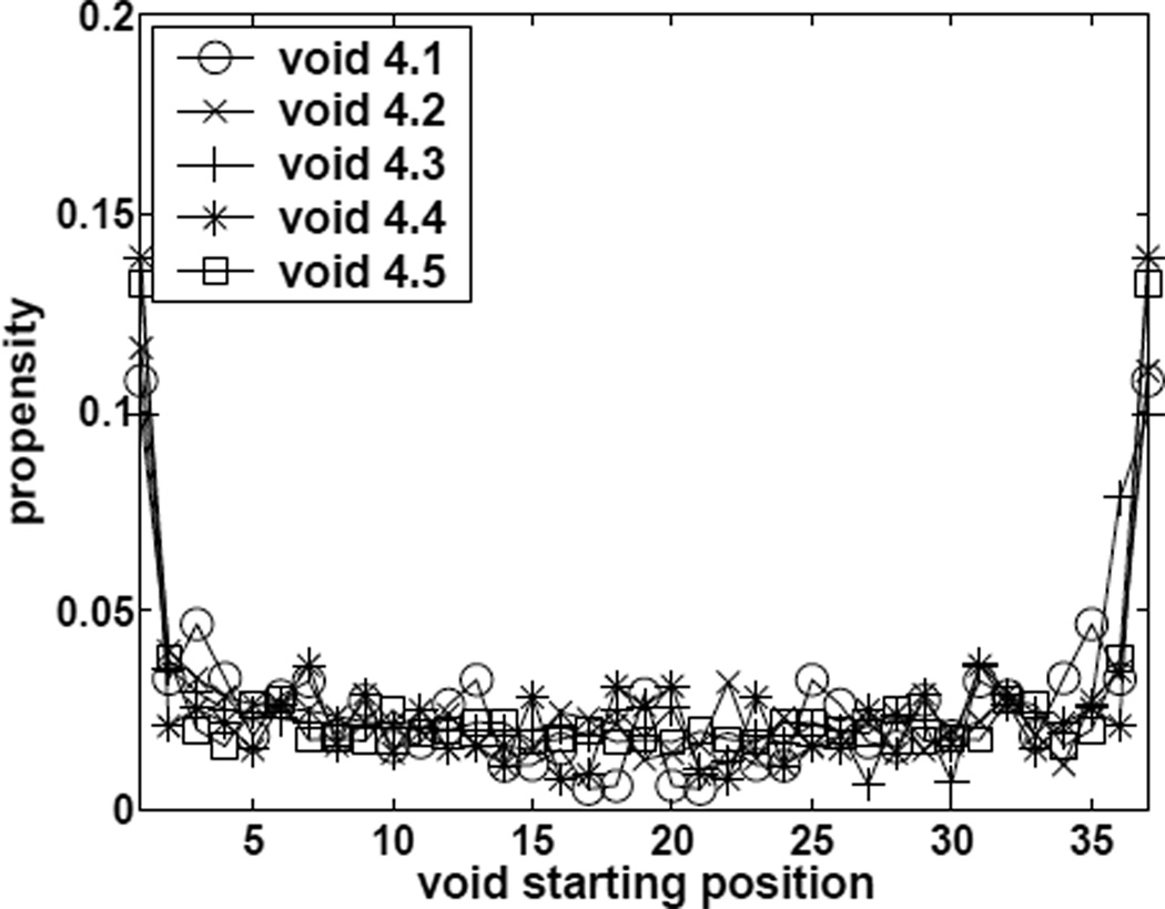
For propensity of void formation with fixed loop length and specified starting position f₃(I₀, l, S, n) as defined in Eqn (3), we plot estimated f₃(I₀, l = 14, S, n = 50) for voids of shapes S with a loop length of 14 in chain polymers of length 50 with different starting positions I₀ in Figure 10. We find that the propensities f₃(I₀, l, S, n) at I₀ = 1 and I₀ = 2 are very different, indicating strong end-effect for void formation. That is, void is much easier to form at the end of the conformation. This is likely due to the tail effect. Void at the end of the chain only need to have one tail, but has two tails if it is in the middle of the conformation. It is difficult to constrain the tails to satisfy the multiple restrictions for forming void of certain shapes.

Fig 10.

Estimated propensity values of forming size-4 voids of different specific shapes with fixed loop length l = 14 and different specified starting position for conformations of length n = 50.

D. Propensity of void formation at different compactness

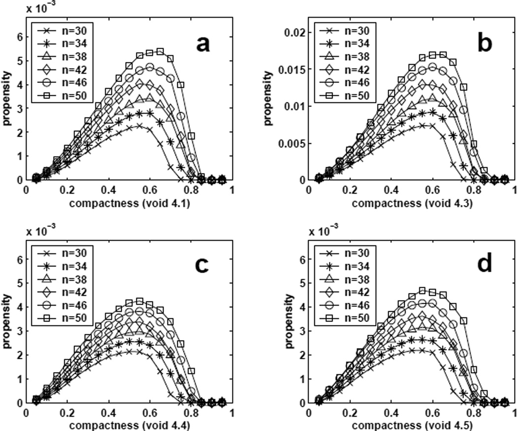
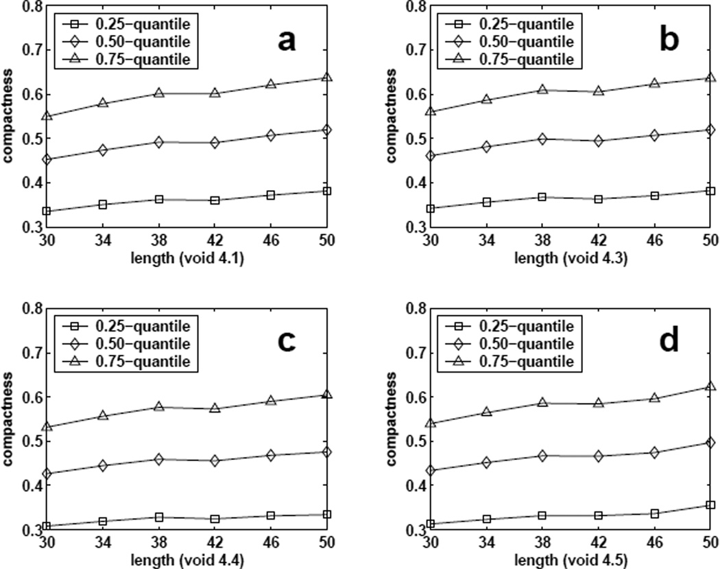
Figure 11 shows estimated propensity values of void formation at different compactness f₄(ρ, S, n) defined in Eqn (4) for chain length from n = 30 to 50. Conformations with size-4 voids are dominated by those at compactness around 0.3 − 0.7. If we normalize f₄(ρ, S, n = 50), that is, we define

$${\mathrm{f̅}}_4(\rho ,S,n)=\frac{f_4(\rho ,S,n)}{\int f_4(\rho ,S,n)d\rho },$$

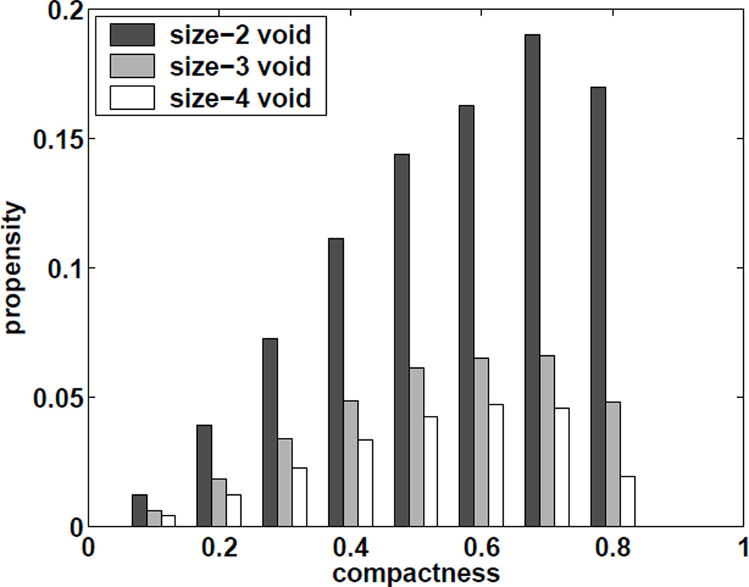
where f̅₄(ρ, S, n) can be considered as a distribution of ρ. We plot the 0.25-quantile, median value, and 0.75-quantile of distribution f̅₄(ρ, S, n) for different chain length n and fixed shape S in Figure 12. We can see these values slightly increase as n increases from 30 to 50. This indicates that the prefer compactness range of forming these size-4 voids shift slightly to more compact regions as chain length increases. We also compare the propensity values of forming voids of all size-2 regular shapes (2.1), voids of all size-3 regular shapes (3.1, 3.2), and voids of all size-4 regular shape (4.1, 4.2, 4.3, 4.4, 4.5) for chains of length 50 at different compactness (Figure 13). The results show that smaller voids are easier to form as compactness increases. Our results from lattice model suggests that there might be a preferred size for void formation in proteins, which are all within a specific narrow range of compactness³.

Fig 11.

Estimated propensity values of forming size-4 voids of different specific shapes with certain compactness for conformations of length from n = 30 to 50. (a–d) : void 4.1, void 4.3, void 4.4, and void 4.5.

Fig 12.

Estimated quantiles (0.25, 0.5, and 0.75) of distribution f̅₄(ρ, S, n) for different chain length n and void shape S. (a–d) : void 4.1, void 4.3, void 4.4, and void 4.5.

Fig 13.

Estimated propensity values of forming voids of all size-2 regular shapes (2.1), voids of all size-3 regular shapes (3.1, 3.2), and voids of all size-4 regular shape (4.1, 4.2, 4.3, 4.4, 4.5) for chain length 50 and different compactness.

IV. SUMMARY AND CONCLUSION

Protein molecules contain many voids buried in the interior of proteins, with broad distribution⁴. Although most voids are likely to originate from generic steric constraints of compact chain polymers^4,5, some voids are the functional regions for many proteins, such as enzymes, where substrates and ligands bind, and biochemical reactions occur^6,7.

An important general question is how the need for maintaining functional voids, which have to be of specific shape, is influenced by, and affects other aspects of proteins structures and properties: e.g., protein folding stability, kinetic accessibility, and evolutionary selection pressure. These are broad and complex issues that require detailed studies.

In this work, we study the effects of maintaining voids of defined shape using lattice model. Because the conformational space of simplified polymers can be examined in detail, lattice models have been widely used in protein studies and have lead to important insight about protein folding. The focus of our study is to generate large number of sample conformations under very constraining restrictions to study general properties of voids and their shapes. We use sequential Monte Carlo method and have developed an efficient growth method to generate conformation samples in highly-constrained space.

We show that our approach is effective in estimating entropy of void maintenance, with and without an increasing number of restrictive conditions, such as loops forming the wall of void with fixed length, with additionally fixed starting position in the sequence. Our results also lead to a number of observations, including that polymers of certain compactness range favors the formation of voids of specific size, and that voids are far easier to form around the end of the polymer. A finding is that voids tend to form at the chain ends. This raises the interesting question whether voids and pockets tend to form at either the N-terminal or the C-terminal end in real proteins. A detailed analysis of voids and pockets in real proteins will be necessary for answering this question. In addition, we have developed a parametric model for explaining the propensity of forming voids of particular shapes, or equivalently, the entropic cost of maintaining such voids. Our model is highly effective in predicting the propensity of void formation for different shapes. Such lattice model of voids representing functional sites can be used as improved model for studying the evolution of protein functions²⁶, and how it relates to protein stability²⁷.

Although in this study we treat the occurrence of all conformations equally likely, our approach can be applied to models with more realistic energy functions in a straight-forward manner. The approach for sampling strongly constrained conformations we developed in this study will be generally applicable for studying real proteins in three-dimensional space.

References

- 1.Richards FM. Ann. Rev. Biophys. Bioeng. 1977;6:151. doi: 10.1146/annurev.bb.06.060177.001055. [DOI] [PubMed] [Google Scholar]
- 2.Chothia C. Nature. 1975;254:304. doi: 10.1038/254304a0. [DOI] [PubMed] [Google Scholar]
- 3.Richards FM, Lim WA. Q. Rev. Biophys. 1994;26:423. doi: 10.1017/s0033583500002845. [DOI] [PubMed] [Google Scholar]
- 4.Liang J, Dill KA. Biophys. J. 2001;81:751. doi: 10.1016/S0006-3495(01)75739-6. [DOI] [PMC free article] [PubMed] [Google Scholar]
- 5.Zhang J, Chen R, Tang C, Liang J. J. Chem. Phys. 2003;118:6102. [Google Scholar]
- 6.Laskowski RA, Luscombe NM, Swindells MB, Thornton JM. Protein Science. 1996;5:2438. doi: 10.1002/pro.5560051206. [DOI] [PMC free article] [PubMed] [Google Scholar]
- 7.Liang J, Edelsbrunner H, Woodward C. Protein Science. 1998;7:1884. doi: 10.1002/pro.5560070905. [DOI] [PMC free article] [PubMed] [Google Scholar]
- 8.Binkowski TA, Adamian L, Liang J. J. Mol. Biol. 2003;332:505. doi: 10.1016/s0022-2836(03)00882-9. [DOI] [PubMed] [Google Scholar]
- 9.Tseng Y, Liang J. Mol. Biol. Evol. 2006;23(2):421. doi: 10.1093/molbev/msj048. [DOI] [PubMed] [Google Scholar]
- 10.Lau KF, Dill KA. Macromolecule. 1989;93:6737. [Google Scholar]
- 11.Chan HS, Dill KA. Macromolecules. 1989;22:4559. [Google Scholar]
- 12.Chan HS, Dill KA. J. Chem. Phys. 1990;92:3118. [Google Scholar]
- 13.Shakhnovich E, Gutin A. J. Chem. Phys. 1990;93:5967. [Google Scholar]
- 14.Camacho CJ, Thirumalai D. Proc. Natl. Acad. Sci. USA. 1993;90:6369. doi: 10.1073/pnas.90.13.6369. [DOI] [PMC free article] [PubMed] [Google Scholar]
- 15.Pande VS, Joerg C, Grosberg AY, Tanaka T. J. Phys. A. 1994;27:6231. [Google Scholar]
- 16.Socci ND, Onuchic JN. J. Chem. Phys. 1994;101:1519. [Google Scholar]
- 17.Dill K, Bromberg S, Yue K, Fiebig K, Yee D, Thomas P, Chan H. Protein Science. 1995;4:561. doi: 10.1002/pro.5560040401. [DOI] [PMC free article] [PubMed] [Google Scholar]
- 18.Lu H, Liang J. Proteins. (Accepted). [Google Scholar]
- 19.Šali A, Shakhnovich EI, Karplus M. Nature. 1994;369:248. doi: 10.1038/369248a0. [DOI] [PubMed] [Google Scholar]
- 20.Shrivastava I, Vishveshwara S, Cieplak M, Maritan A, Banavar JR. Proc. Natl. Acad. Sci. U.S.A. 1995;92:9206. doi: 10.1073/pnas.92.20.9206. [DOI] [PMC free article] [PubMed] [Google Scholar]
- 21.Klimov DK, Thirumalai D. Phys. Rev. Lett. 1996;76:4070. doi: 10.1103/PhysRevLett.76.4070. [DOI] [PubMed] [Google Scholar]
- 22.Mélin R, Li H, Wingreen N, Tang C. J. Chem. Phys. 1999;110:1252. [Google Scholar]
- 23.Kachalo S, Lu H, Liang J. Phys Rev Lett. 2006;96(5) doi: 10.1103/PhysRevLett.96.058106. 058106. [DOI] [PubMed] [Google Scholar]
- 24.Liang J, Zhang J, Chen R. J. Chem. Phys. 2002;117:3511. [Google Scholar]
- 25.Zhang J, Chen Y, Chen R, Liang J. J. Chem. Phys. 2004:592–603. doi: 10.1063/1.1756573. [DOI] [PubMed] [Google Scholar]
- 26.Williams PD, Pollock DD, Goldstein R. Journal of Molecular Graphics and Modelling. 2001;19:150. doi: 10.1016/s1093-3263(00)00125-x. [DOI] [PMC free article] [PubMed] [Google Scholar]
- 27.Bloom JD, Wilke CO, Arnold FH, Adami C. Biophys. J. 2004;86:2758. doi: 10.1016/S0006-3495(04)74329-5. [DOI] [PMC free article] [PubMed] [Google Scholar]
- 28.Rosenbluth MN, Rosenbluth AW. J. Chem. Phys. 1955;23:356. [Google Scholar]
- 29.Gilks WR, Richardson S, Spiegelhalter DJ. Markov Chain Monte Carlo in Practice. Chapman & Hall; 1996. [Google Scholar]
- 30.Hamelryck T, Kent J, Krogh A. PLoS Comput. Biol. 2006;2:1121. doi: 10.1371/journal.pcbi.0020131. [DOI] [PMC free article] [PubMed] [Google Scholar]
- 31.Iba Y, Chikenji G, Kikuchi M. Journal of the Physical Society of Japan. 1998;67:3327. [Google Scholar]
- 32.Chan HS, Dill KA. J. Chem. Phys. 1989;90:492. [Google Scholar]
- 33.Marshall A. In: Meyer M, editor. Symposium on Monte Carlo Methods; Wiley; 1956. pp. 123–140. [Google Scholar]
- 34.Liu JS. Monte Carlo Strategies in Scientific Computing. New York: Springer; 2001. [Google Scholar]
- 35.Grassberger P. Phys. Rev. E. 1997;56:3682. [Google Scholar]
- 36.Zhang JL, Liu JS. J. Chem. Phys. 2002;117:3492. [Google Scholar]
- 37.Fearnhead P, Clifford P. J.R.Statist. Soc. B. 2003;65:887. [Google Scholar]
- 38.Hatcher A. Algebraic topology. Cambridge, England: Cambridge University Press; 2002. [Google Scholar]
- 39.Meirovitch H. J. Phys.A: Math. Gen. 1982;15:L735. [Google Scholar]
- 40.Wang X, Chen R, Guo D. IEEE trans. Signal Processing. 2002;50:241. [Google Scholar]
- 41.Kong A, Liu J, Wong W. J. Amer. Statist. Assoc. 1994;89:278. [Google Scholar]