Abstract
The basic principle of graph-based approaches for image segmentation is to interpret an image as a graph, where the nodes of the graph represent 2D pixels or 3D voxels of the image. The weighted edges of the graph are obtained by intensity differences in the image. Once the graph is constructed, the minimal cost closed set on the graph can be computed via a polynomial time s-t cut, dividing the graph into two parts: the object and the background. However, no segmentation method provides perfect results, so additional manual editing is required, especially in the sensitive field of medical image processing. In this study, we present a manual refinement method that takes advantage of the basic design of graph-based image segmentation algorithms. Our approach restricts a graph-cut by using additional user-defined seed points to set up fixed nodes in the graph. The advantage is that manual edits can be integrated intuitively and quickly into the segmentation result of a graph-based approach. The method can be applied to both 2D and 3D objects that have to be segmented. Experimental results for synthetic and real images are presented to demonstrate the feasibility of our approach.
Keywords: Segmentation, Graph-based, Manual refinement, 2D, 3D
Introduction
Image segmentation is the process of partitioning a digital image into several segments to simplify and change the representation of an image into something more meaningful and easier to analyze [1]. In particular, medical image segmentation is becoming progressively more important [2], since medical patient data is becoming more detailed and today’s computers are able to process large amounts of medical image data within a reasonable time. Several segmentation algorithms ranging from simple threshold methods to high-level segmentation approaches have been proposed in the literature [3]. For example, high-level segmentation approaches are deformable methods such as Active Contours (ACM) in 2D [4] and in 3D [5]. Additionally, there are statistical approaches such as Active Appearance Models (AAM) [6, 7] which use the shape [8] and the texture [9] of an object to perform image segmentation. A third class of high-level segmentation methods consists of graph-based approaches that interpret an image as a graph with nodes and edges [10, 11, 12]. To perform a segmentation after a graph has been constructed, the minimal cost closed set on the graph can be computed via a polynomial time s-t cut [13], separating the object from the background. However, no segmentation method provides a perfect result, and additional editing is always required in the current approaches. This is the main reason why several algorithms for interactive segmentation have been proposed. Vezhnevets and Konouchine [14] provided an overview of methods for generic and medical image editing and presented an algorithm for interactive multilabel segmentation of N-dimensional images. The segmentation process is iterative and works with a small number of user-labeled pixels to segment the rest of the image automatically by a Cellular Automaton, This algorithm has been incorporated into the medical platform Slicer (see http://www.slicer.org/) as a module and therefore can be easily tested [15]. An interactive segmentation technique called Magic Wand [14] is a common selection tool for almost any image editor today. The tool gathers color statistics from the user specified image point (or region) and segments (connected) image regions with pixels whose color properties fall within some given tolerance of the gathered statistics. Reese [16] presented a region-based interactive segmentation technique, based on hierarchical image segmentation by tobogganing, which uses a connect-and-collect strategy to define an object’s region. The so-called Intelligent Paint uses a hierarchical tobogganing algorithm to automatically connect image regions that naturally flow together, and a user-guided, cumulative costordered expansion interface to interactively collect the regions that constitute the object of interest. Mortensen and Barrett [17] introduced a boundary-based method that computes a minimum-cost path between user-specified boundary points. The intelligent scissors method treats each pixel as a graph node and uses shortest-path graph algorithms for boundary calculation, while the faster variant of region-based intelligent scissors uses tobogganing for image over-segmentation and then treats homogenous regions as graph nodes [18]. GraphCut, is a combinatorial optimization technique applied to the task of image segmentation by Boykov and Jolly [19]. Here, the image is treated as a graph and the technique can be applied to N-dimensional images. Given user-specified object and background seed pixels, the rest of the pixels are labeled automatically. An extension of the GraphCut, named GrabCut, has been developed by Rother et al. [20], where an iterative segmentation scheme uses a graph-cut for intermediate steps. In the presented approach, the user draws a rectangle around the object of interest as a first approximation of the final object and background labeling. Subsequently, each iteration step gathers color statistics according to the current segmentation, re-weights the image graph and applies a graph-cut to compute a refined segmentation. When the iterations stop, the segmentation results can be refined by specifying additional seeds, similar to the original graph-cut. A marker-based watershed transformation algorithm for medical image segmentation has been developed by Moga and Gabbouj [21] that uses user-specified markers for segmenting gray level images. Watershed transform methods treat an image as a surface with the relief specified by the pixel brightness or by the absolute value of the image gradient. Afterwards, the valleys of the resulting landscape are filled with water, until the mountains are reached. The markers that are placed in the image specify the initial labels that should be segmented. The random walker algorithm of Grady and Funka-Lea [22] is a probabilistic approach where a small number of pixels with user-defined seed labels (label numbers can be greater than two) are given. Then, the approach analytically determines the probability that a random walker starting at each unlabelled pixel will first reach one of the pre-labeled pixels. Image segmentation is obtained by assigning each pixel to the label for which the greatest probability is calculated, and additionally a confidence rating of each pixel’s membership in the segmentation is estimated. Heimann et al. [23] demonstrated an interactive region growing method, a descendant of one of the classic image segmentation techniques. The method works only with two labels, object and background and the seed pixel inside the object of interest is specified at the beginning. Neighboring pixels are then iteratively added to the growing region while conforming to defined region homogeneity criteria. Leaking is the main problem of the growing region through weak boundaries of the object. However, several solutions to this problem have been proposed.
An evaluation of the above described methods by Rother et al. [20] has shown that methods based on graph-cuts allow us to achieve better segmentation results with less user effort required compared with other methods. However, one of the few drawbacks of graph-based methods is that they are not very flexible. The only tunable parameters are the graph weighting and cost-function coefficients, e.g. additional restrictions on the object boundary smoothness or soft user-specified segmentation constraints cannot be added easily [14].
In this paper, we present an approach to avoid this drawback by taking advantage of the basic design of graph-based segmentation algorithms. Our approach restricts a graph-cut by using additional user-defined seed points to set up fixed nodes in the graph. The advantage of this approach is that manual edits can be integrated intuitively and quickly into the segmentation result of a graph-based approach. The method can be applied for segmentation of both 2D and 3D objects. Experimental results for synthetic and real images are presented to demonstrate the feasibility of our approach.
The paper is organized as follows. “Material and methods” describes the used material, the newly proposed approach and the theoretical background of the developed algorithm. In “Results”, experimental results are presented. “Discussion” discusses the significance of the presented results and outlines areas for further work.
Material and methods
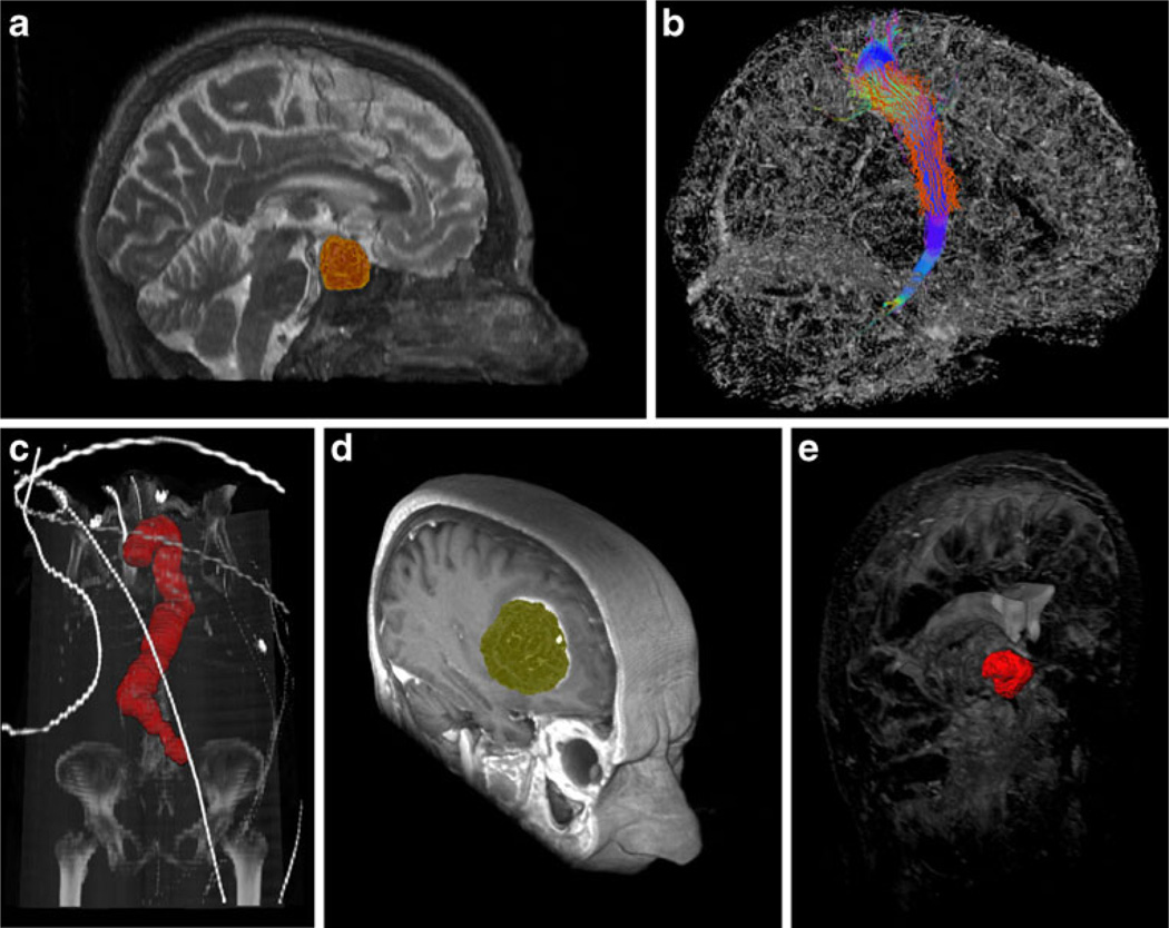
In the medical field, we have used graph-based segmentation approaches for pituitary adenoma in magnetic resonance imaging (MRI) data [24, 25], fiber tracts in Diffusion Tensor Imaging (DTI) data [26, 27, 28], abdominal aortic aneurysms (AAA) in computed tomography angiography (CTA) data [29, 30, 31], glioblastoma multiforme (GBM) in MRI data [32, 33, 34], and cerebral aneurysm in computed tomography (CT) data [35]. Figure 1 shows several segmentation results as 3D screenshots faded into whole image structures. The upper left image (a) is a pituitary adenoma segmented from a MRI scan. The upper right image (b) shows a sagittal view of the right corticospinal tract with calculated boundary (red) from a DTI scan. The left image in the lower row (c) shows a segmentation of the entire aorta including an abdominal aortic aneurysm from a CTA scan. This segmentation has been achieved with an iterative graph-based approach that tracks along the centerline. The middle image of the lower row (d) presents the segmentation result of a glioblastoma multiforme (GBM) in a MRI scan. Finally, the right image of the lower row (e) displays the segmentation result of a cerebral aneurysm from a computed tomography (CT) scan.
Fig. 1.
Examples from medical applications where we have used graph-based image segmentation approaches. Upper row from the left: pituitary adenoma (MRI) (a), fiber tracts (DTI) (b). Lower row from the left: aorta with abdominal aneurysm (CTA) (c), glioblastoma multiforme (MRI) (d), cerebral aneurysm (CT) (e)
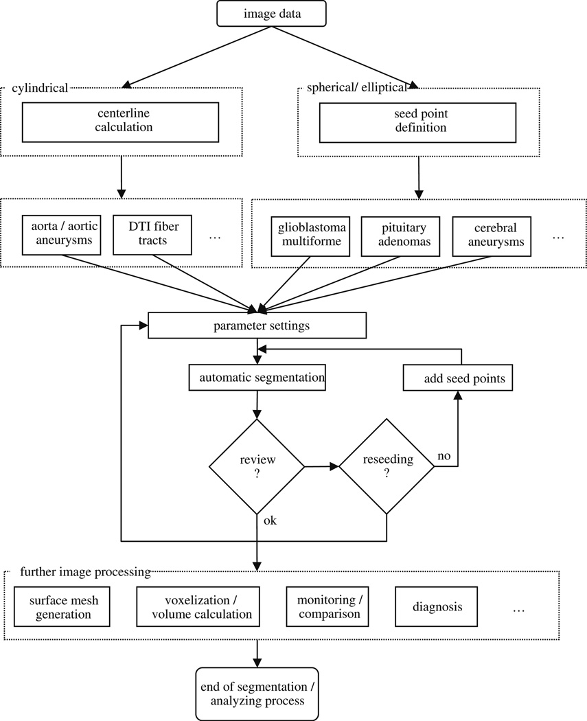
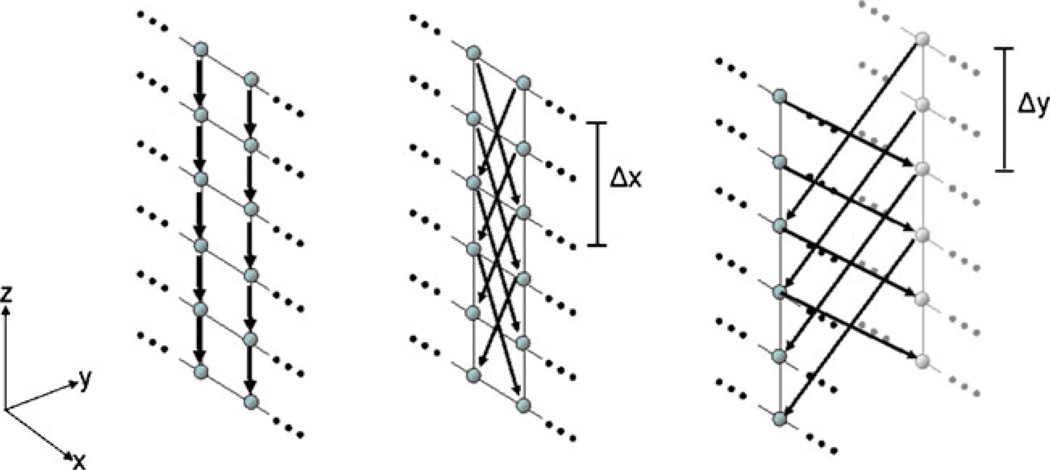
The global workflow of our manual refinement method is shown in Fig. 2. The method starts with 2D or 3D image data. Identification of a certain pathology leads to specific parameter settings by the user that is stored in the system. As such, it must be decided if a more spherically or elliptically shaped object like a pituitary adenoma or a cylindrical object like the aorta has to be segmented. In case of a cylindrical object, an initial centerline [36] for the graph-based approach is needed. For spherically shaped objects, only a single user-defined seed point somewhere inside the lesion is required in addition to the predefined parameter settings. The predefined parameter setting can be a specific segmentation diameter. For example, the segmentation diameter of cerebral aneurysms would be much smaller than the diameter for the segmentation of GBM. Pituitary adenomas are more spherically shaped than GBMs and, therefore, the stiffness parameter chosen would be smaller for pituitary adenomas. After the initial seed point or centerline has been defined and the parameters set, automatic segmentation starts and calculates the lesion’s boundary. The algorithm for automatic segmentation is based on a novel graph-based scheme that has recently been developed for spherically and elliptically shaped objects [32] and an iterative graph-based approach for cylindrical objects [30]. To summarize, the schemes create a directed 3D graph for both cases by (1) sending out rays and (2) sampling the graph’s nodes along every ray. Thereafter, the minimal cost closed set on the graph is computed via a polynomial time s-t, cut [13], creating an optimal segmentation of the lesion’s boundary. The sampled points are the nodes v∈Vof the graph G(V,E), and e∈E is the corresponding set of edges. There are edges between the nodes and edges that connect the nodes to a source node s and a sink node t, to allow the computation of an s-t, cut (note: the source and the sink s, t∈V are, virtual nodes). The arcs< vi, vj > ∈E, of the graph G, connect two nodes vi, vj, For cylindrical objects, there are three types of ∞-weighted arcs: z arcs (Az), x-z, arcs (Axz),, and y-z, arcs (Ayz), (X, is the number of rays sent out radially (x=0,…,X-1), Y the number of planes (y=0,…,Y-1) along the centerline and Z the number of sampled voxels along one ray (z=0,…,Z-1)), (see Fig. 3):
| (1) |
| (2) |
| (3) |
Fig. 2.
The overall workflow of the proposed system; it starts with the image data and ends with the image segmentation and analysis process
Fig. 3.
The three different types of arcs for a graph that is used to segment cylindrically shaped objects. Left: Az arcs. Middle: Axz arcs. Right: Ayz arcs [29]
Equation 1 describes the intracolumn arcs Az, which ensure that all nodes below the surface in the graph are included to form a closed set (correspondingly, the interior of the cylindrical object is separated from the exterior in the original plane). In Fig. 3 the intracolumn arcs Az, – and their directions – are shown on the left side (black arrows downward-pointing). The Eqs. 2 and 3 describe the intercolumn arcs Axz, and Ayz, which constrain the set of possible segmentations and enforce smoothness via two delta parameters Δx and Δy. The larger these parameters are, the larger is the number of possible segmentations. In Fig. 3 the intercolumn arcs Axz, are shown in the middle and the intercolumn arcs Ayz, are shown on the right side – both, the arcs and their directions are illustrated by black arrows in the images.
For spherically or elliptically shaped objects there are two types of ∞-weighted arcs: z-arcs Az, and r-arcs Ar, (Z is the number of sampled points along one ray z=(0,…,Z-1), and R, is the number of rays sent out to the surface points of a polyhedron r=(0,…,R-1)),, where V(xn,yn,zn), is one neighbor of V(x,yz), – in other words V(xn,yn,zn), and V(x,yz), belong to the same triangle in case of a triangulation of the polyhedron (with Ar, as stiffness parameter):
| (4) |
| (5) |
The weights w(x, y z), for every edge between v∈V, and the sink or source are assigned in the following manner: weights are set to c(x,y,z), when z is zero and otherwise to c (x,y,z)-c(x,y,z-1),, where c(x,y,z), is the absolute value of the intensity difference between an average gray value of the desired object and the grey value of the voxel at position (x,y,z).
After the automatic segmentation has been performed, the user reviews the result. If the result is not satisfactory, there are two possibilities for the user: (1) delete the seed point or the centerline and start over with a new seed point or centerline that is, for example, located closer to the center of the lesion and therefore leads to a better segmentation result, or (2) add an arbitrary number of seed points to support the algorithm. The user can add seed points on the object boundary that has been under- or over-segmented. These seed points ensure that the resultant border contains these user-defined restrictions when the automatic segmentation is performed again. Subsequently, further image processing can be done. This might be the generation of a surface mesh to perform an additional voxelization and volume calculation of the object. In the medical field, this can be used for monitoring or diagnosing a pathology, which is a very time-consuming process if performed manually (a detailed description follows in the “Results” section).
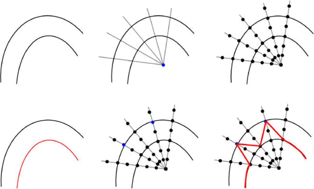
Figure 4 demonstrates the principle of how additional seed points affect the global segmentation result. The left image of the upper row shows some structures in an image, where the goal is to segment the outer boundary. The middle image of the upper row illustrates how rays are sent out from a user-defined seed point (blue) to prepare the graph construction. Along these rays, the nodes for the graph (black dots) are sampled as shown in the upper right image. However, the segmentation results returned the inner boundary (red) because of higher intensity values (see lower left image). In the middle image of the lower row, two additional seed points (blue) are provided to the algorithm, and with these additional seed points, the outer boundary will be returned by the algorithm. A result that still includes some parts of the inner boundary as shown in the lower right image (red) is not possible, because the additional seed points also affect the neighbor nodes via the delta value. Note that for illustration purposes, only a few nodes were sampled along the rays, and in the example, the nodes sit on the boundaries. For implementation of the algorithm, a much higher sampling rate has to be chosen. Otherwise, there will be rays that do not provide sampled nodes located directly on the object’s border. If the user then adds a seed point, it has to be decided which node has to be fixed in the graph, e.g. via the shortest Euclidean distance from the user’s seed point to a graph node. However, this would also mean that the cut would not be located exactly along the object’s border as wanted by the user.
Fig. 4.
The principle how additional seed points affect the global segmentation result. Upper Row: some structures in an image, where the goal is to segment the outer boundary (left). Rays are sent out from a user-defined seed point (blue) to prepare the construction of the graph (middle). Nodes for the graph (black dots) are sampled along the rays (right). Lower Row: Segmentation returned the inner boundary (red) due to higher intensity values (left). Two additional seed points (blue) are provided (middle). The additional seeds will return the outer boundary. A result that still includes some parts of the inner boundary (red) is not possible because the additional seeds also affect the neighbor nodes (right)
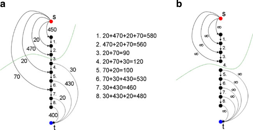
Figure 5 illustrates the principle when the user adds seed points on the object’s boundary that has been under- or over-segmented by the graph-based algorithm. The additional seed points ensure that the resulting border contains the user-defined restrictions when the automatic segmentation is performed again. Image A on the left side of Fig. 5 shows a small graph that consists of several nodes and arcs. There are intracolumn arcs between two nodes along the ray that ensure that all nodes below the segmented surface in the graph are included to form a closed set. Correspondingly, the interior of the object is separated from the exterior in the data. Furthermore, there are arcs connecting the nodes to the source s and the sink t. The weights of the arcs connecting the nodes with the source and the sink depend on gray value difference between two adjacent nodes in the image. A typical cut (green line) for the example in Fig. 5 would remove the third arc, so the upper three nodes belong to the source s and define the background, and the lower six nodes belong to the sink t and define the object (and the object boundary lies at the third arc). For all possible eight cuts, the costs are also presented in Fig. 5. The lowest cut has a cost of ninety, and this is the reason why the third intracolumn arc is removed by performing the s-t cut. However, as mentioned previously, no segmentation scheme provides perfect results, and thus the user might want to have the cut going through the fourth arc. When reviewing the segmentation result, the user can set an additional seed point in the area of the fourth arc. To accomplish this additional geometrical restriction, the fourth arc is removed during graph construction, or rather is not generated at all. In addition, the upper four nodes are bound with a maximum weight to the source s and the lower five nodes are bound with a maximum weight to the sink t. This definitely forces the s-t, cut (green line) to run between the fourth and the fifth node, as shown in Image 4 on the right side (B). This restriction also influences the adjacent nodes and rays. Due a small stiffness value (e.g. a delta value Δ less than three), the specific cut for this ray would not allow a cut on an adjacent ray that lies, for example, between node one and node two. This would be a conflict between the allowed resulting surfaces (predefined by the delta value) and the user restricted cut, and, therefore, the s-t cut will avoid it automatically. For segmentation on image data this is reasonable, because an object border will not increase too much between two adjacent rays. If the user provides the algorithm with an extra seed point on the object border, this means that the adjacent part of the object border is located in a similar region. In the medical field this makes even more sense, since an aneurysm or tumor boundary will not “jump”, between two adjacent points on the boundary.
Fig. 5.
Left side a: an example of performing a graph-based cut (green line) for specific arcs between nodes (intracolumn) and arcs to the source s and the sink t, with certain weights gained from an image. An example of forcing the cut (green line) to occur between two specific nodes by (1) removing the intracolumn arc between the two nodes, and (2) binding the upper four nodes with unlimited weights to the source s and the lower five nodes with unlimited weights to the sink t [35]
Various interactive segmentation methods from the literature, presented in the state of the art paragraph of this publication, integrate the intensity values from the additional seeds and labels provided by the user. This can also be done for the currently proposed method. Thus, the algorithm can be supported with both intensity value information and geometrical constraints.
Results
To implement the presented segmentation algorithm and manual refinement method, the medical prototyping platform MeVisLab (http://www.mevislab.de) has been used; and the algorithm has been implemented in C++ as an additional MeVisLab module. Although the MeVisLab Platform has been developed for medical applications, it is also possible to process images from other fields. Even when the graph-cut was performed with several manually defined fixed nodes, the overall segmentation for our implementation took only about one second on an Intel Core i5-750 CPU, 4×2.66 GHz, 8 GB RAM, Windows XP Professional x64 Version, Version 2003, Service Pack 2.
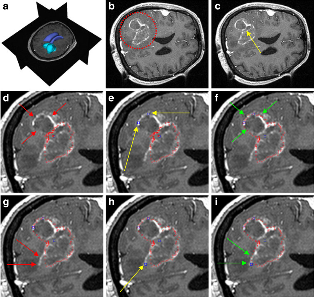
For our evaluation, we used synthetic and real images. However, the focus was on real medical patient data from clinical routine scans, where ground truth data was available. The ground truth (GT) data was extracted by manual slice-by-slice segmentations by physicians. Figure 6 presents the principle of using the manual refinement method for an under-segmented GBM in a MRI scan. The under-segmentation resulted from a graph-based approach that used only one user-defined seed point inside the GBM. The first image in the upper row (A) shows a 3D visualization of the MRI dataset that was used for segmentation, with the tumor in turquoise and the ventricle in blue. Image B displays an axial multiplanar reformatting (MPR) slice of the MRI dataset where the location of the GBM is surrounded by a red circle. The following image C includes a yellow arrow that points to the position of the user-defined seed point inside the GBM. This seed point is the only manual information provided to the graph-based segmentation approach. In the next image D, red spots superimpose the segmentation result. Additionally, two red arrows mark the GBM boundary that has not been segmented by the graph-based algorithm. There are three main reasons why under-segmentation occured for this image. First, segmentation results are based not only on a single slice but rather acts in 3D; therefore, the adjacent slices also affect the segmentation result. Second, in this case the tumor was not spherical or elliptical; therefore, although mimicking a real-life situation, it was not the ideal case for the segmentation algorithm. Third, in addition to the outer GBM boundary that we want to segment, an inner boundary exists. In this case, the inner boundary was preferred by the algorithm. In Fig. 4, we have the same situation: an inner and an outer boundary with similar intensity values exist, and the algorithm favors the inner boundary. The solution for such a case is integrating additional nodes to force the graph-cut towards a certain boundary. Thus, after the segmentation result is provided to the user, additional seed points can be added to support the graph-based algorithm. In this case, two additional user-defined seed points (blue) along the contrast enhanced GBM boundary are set (E). Yellow arrows display the exact positions of these seed points. The following image (F) presents the segmentation results (red spots) after the additional seed points have been included into the graph and the cut has been performed again. The green arrows in the image point out the updated GBM boundary. However, for this example the GBM boundary has not been segmented perfectly. There is still an area where the algorithm missed the GBM contour (see the red arrows in image G). Therefore, the user placed an additional user-defined seed point (blue) along the contrast enhanced GBM boundary (yellow arrow) as shown in image H. The next image I shows the final segmentation result (red spots) after three additional seed points have been placed on the image and included in the graph. The green arrows indicate the new boundary around the last seed that has been included in the graph. This example is a step-by-step illustration. Of course, the user can add all three additional seed points at the same time after the first segmentation result has been provided. It is not necessary to add two seed points, perform the segmentation and thereafter add another seed point and perform the segmentation again.
Fig. 6.
The principle of using the manual refinement method for an under-segmented glioblastoma multiforme (GBM) in a MRI scan. a: 3D visualization of the MRI dataset with the tumor in turquoise and the ventricle in blue (performed with Slicer, see http://www.slicer.org/). b: location of the GBM (red circle). c: position of the user-defined seed point inside the GBM (yellow arrow). d: segmentation result (red spots) and missed GBM boundary (red arrows). e: position of two additional user-defined seed points (blue) along the GBM boundary (yellow arrows). f: segmentation results (red spots) after the additional seed points have been included into the graph (green arrows). g: missed GBM boundary (red arrows). h: position of an additional user-defined seed point (blue) placed along the GBM boundary (yellow arrow). i: final segmentation results (red spots) after three additional seed points have been placed on the image and therefore included into the graph. Green arrows indicate the new boundary around the last seed that has been included into the graph
The next four tables present detailed evaluation results of the presented method for twelve GBM cases. For every case, the volume (cm3) and number of voxels are provided(see Table 1). The ground truth (GT) has been extracted by physicians. The second columns under the volume, and the number of voxel, headings show the segmentation results when the graph-based approach has been performed with one seed (OS) point located inside the GBM. The third columns present the results of the manual refinement (MR) method for all cases where restricted nodes during the graph construction have been set up. The last two columns of the whole table present the results of the Dice Similarity Coefficient (DSC) [37] and [38] between the ground truth and the one seed segmentation (DSCOS) and the ground truth and the manual refinement method DSCmr). The Dice Similarity Coefficient is the relative volume overlap between A, and R:
| (6) |
where A, and R, are the binary masks from the automatic (A) and the reference (R), segmentation. V(·) is the volume (in cm3) of voxels inside the binary mask, by means of counting the number of voxels, then multiplying with the voxel size. The summary of results (volume, number of voxel, DSCOS and DSCmr): min, max, mean µ and standard deviation σ for all cases is presented in Table 2 and Table 3, so the global improvement gets obvious.
Table 1.
Segmentation results for twelve glioblastoma multiforme: ground truth (GT) that has been extracted by the physicians, one seed (OS) used for performing automatic segmentation and manual refinement (MR) by setting up restricted nodes during graph construction
| Case No. | Volume (cm3) |
Number of voxel |
DSCOS (%) | DSCMR (%) | ||||
|---|---|---|---|---|---|---|---|---|
| GT | OS | MR | GT | OS | MR | |||
| 1 | 4721.37 | 5033.78 | 5033.7 | 23470 | 25023 | 25023 | 85.08 | 85.08 |
| 2 | 13055.7 | 8409.35 | 11020.1 | 64900 | 41803 | 54781 | 78.34 | 89.48 |
| 3 | 3067.39 | 1196.5 | 1196.5 | 15251 | 5949 | 5949 | 56.09 | 73.56 |
| 4 | 32946.8 | 29373.4 | 29373.4 | 283011 | 252316 | 252316 | 91.54 | 91.54 |
| 5 | 86914.9 | 65599.5 | 67516.3 | 93324 | 68786 | 72495 | 81.33 | 86.37 |
| 6 | 52536.9 | 39853.2 | 39853.2 | 56411 | 42792 | 42792 | 86.26 | 86.26 |
| 7 | 2382.01 | 2186.07 | 2186.07 | 11841 | 10867 | 10867 | 87.8 | 87.8 |
| 8 | 4332.68 | 4544.06 | 4544.06 | 21542 | 22593 | 22593 | 91.96 | 91.96 |
| 9 | 12005.9 | 5722.87 | 5722.87 | 59693 | 28454 | 28454 | 62.92 | 73.79 |
| 10 | 2694 | 993 | 993 | 2694 | 993 | 993 | 53.76 | 72.61 |
| 11 | 35023 | 21598 | 21355.6 | 35023 | 21598 | 24462 | 76.19 | 82.48 |
| 12 | 2510.22 | 2079.14 | 1899.9 | 20180 | 24364 | 18441 | 81.38 | 85.99 |
Table 2.
Summary of results (volume / number of voxel): min, max, mean µ and standard deviation σ for twelve glioblas-toma multiforme
| Volume (cm3) |
Number of voxel |
|||||
|---|---|---|---|---|---|---|
| GT | OS | MR | GT | OS | MR | |
| min | 2.38 | 0.99 | 0.99 | 2694 | 993 | 993 |
| Max | 86.91 | 65.60 | 67.51 | 283011 | 252316 | 252316 |
| µ±σ | 21.02±26.48 | 15.55±20.18 | 20.31±22.16 | 57278.33 | 45461.5 | 58196.7 |
Table 3.
Summary of results (DSC): min, max, mean µ and standard deviation σ for twelve glioblastoma multiforme
| DSCOS (%) | DSCMR (%) | |
|---|---|---|
| min | 53.76 | 72.61 |
| max | 91.96 | 91.96 |
| µ±σ | 77.72±13.19 | 83.91 ±6.91 |
The manual slice-by-slice segmentation time required to obtain the GT by the physicians is shown in Table 4 for all twelve GBM datasets (mean µ = 8.08 and standard deviation σ = 5.18). This manual segmentation time was compared with the execution time of the algorithm which only took approximately one second in our implementation, as mentioned previously in the beginning of this section.
Table 4.
Manual slice-by-slice segmentation time in minutes of the physicians for twelve glioblastoma multiforme (mean µ = 8.08 and standard deviation σ = 5.18)
| Case No. | 1 | 2 | 3 | 4 | 5 | 6 | 7 | 8 | 9 | 10 | 11 | 12 |
|---|---|---|---|---|---|---|---|---|---|---|---|---|
| Time (min.) | 5 | 11 | 7 | 19 | 16 | 6 | 3 | 4 | 10 | 3 | 9 | 4 |
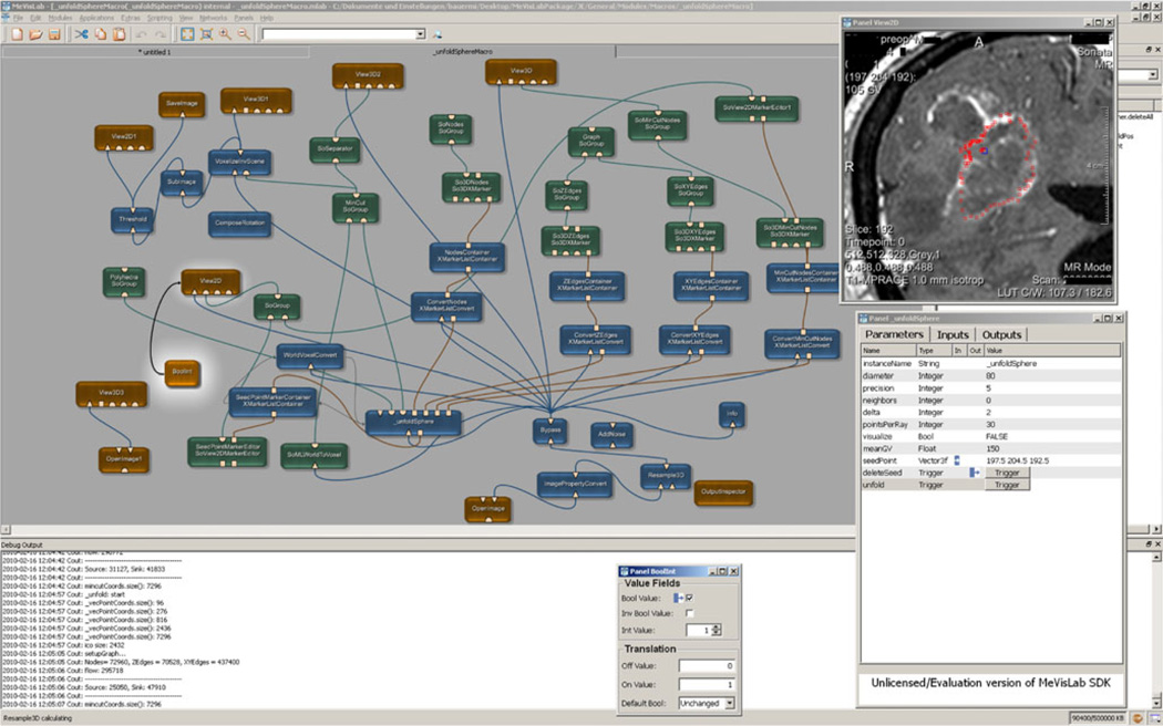
Finally, Fig. 7 presents the modules and connection between the modules that have been used for accomplishing the graph-based algorithm and the manual refinement method for pituitary adenomas, GBM and cerebral aneurysms under the medical prototyping platform MeVisLab.
Fig. 7.
Modules and connections used for the manual refinement method for pituitary adenoma, glioblastoma multiforme and cerebral aneurysm under the medical prototyping platform MeVisLab (see http://www.mevislab.de/)
Discussion
In this study, we have presented a manual refinement method for graph-based segmentation approaches. The method takes advantage of the basic design of graph-based segmentation algorithms. To the best of our knowledge, this is the first application restricting a graph-cut approach by using additional user-defined seed points to set up fixed nodes in the graph. The advantage of this method is that manual edits can be integrated intuitively and quickly into the segmentation results of a graph-based approach. The method is eligible for segmentation of both 2D and 3D objects. Furthermore, this segmentation method can be applied to all kind of objects using the graph-based method; it does not matter if the object is represented by a 2D contour or a 3D surface.
There are several areas of future work. For example, adjustment of the delta parameter of the graph-based algorithm to the distance to a fixed manual node is planned (Table 1). This will allow more perfect results when additional seed points are used for constructing the graph. The cases from Table 1 can then be analyzed to find a regulation for the cases that could not be improved. Additionally, we intend to compare the presented method with the Growcut algorithm of Vezhnevets and Konouchine [14] implemented in Slicer [15] using the same clinical GBM data sets. Furthermore, the method can be enhanced with statistical information about the shape and the texture [39] of the desired object. Finally, idea is to automatically “snap” a seed to the lesion’s boundary if a physician wants to add a seed point. Then, the physician has not to click exactly on the lesion’s boundary, which is sometimes hard when not zoomed in and time consuming when several attempts have to be performed.
Acknowledgements
The authors would like to thank the physicians Dr. Barbara Carl, Christoph Kappus, Dr. Malgorzata Kolodziej and Dr. Daniela Kuhnt for performing the manual segmentations of the medical images and therefore providing the ground truth for the evaluation. Furthermore, the authors want to thank Prof. Dr. Ron Kikinis for his thoughtful comments and Dr. Sonia Pujol for helping performing the 3D visualization of the tumor and the ventricle under Slicer (see http://www.slicer.org/). Finally, the authors would like to thank Fraunhofer MeVis in Bremen, Germany, for their collaboration and especially Prof. Dr. Horst K. Hahn for his support.
Footnotes
Conflict of interest statement All authors in this paper have no potential conflict of interests.
Contributor Information
Jan Egger, Email: egger@bwh.harvard.edu, Surgical Planning Laboratory, Department of Radiology, Brigham and Women’s Hospital, Harvard Medical School, 75 Francis St., Boston, MA 02115, USA; Department of Mathematics and Computer Science, University of Marburg, Hans-Meerwein-Str., 35032 Marburg, Germany; Department of Neurosurgery, University of Marburg, Baldingerstraße, 35043 Marburg, Germany.
Rivka R. Colen, Email: rrcolen@bwh.harvard.edu, Surgical Planning Laboratory, Department of Radiology, Brigham and Women’s Hospital, Harvard Medical School, 75 Francis St., Boston, MA 02115, USA.
Bernd Freisleben, Email: freisleb@informatik.uni-marburg.de, Department of Mathematics and Computer Science, University of Marburg, Hans-Meerwein-Str., 35032 Marburg, Germany.
Christopher Nimsky, Email: nimsky@med.uni-marburg.de, Department of Neurosurgery, University of Marburg, Baldingerstraße, 35043 Marburg, Germany.
References
- 1.Shapiro LG, Stockman GC. Computer vision. Prentice Hall; 2001. p. 608. ISBN 0-13-030796-3. [Google Scholar]
- 2.Pham DL, Xu C, Prince JL. Current methods in medical image segmentation. Annu. Rev. Biomed Eng. 2000;02:315–337. doi: 10.1146/annurev.bioeng.2.1.315. [DOI] [PubMed] [Google Scholar]
- 3.Cufí X, Muñoz X, Freixenet J, Martí J. A review on image segmentation techniques integrating region and boundary information. Adv. Imag. Electron Phys. 2003;120:1–39. [Google Scholar]
- 4.Kass M, Witkin A, Terzopolous D. Snakes: Active contour models. International Journal of Computer Vision (IJCV) 1988;1(4):321–331. [Google Scholar]
- 5.Kass M, Witkin A, Terzopoulos D. Constraints on deformable models: Recovering 3D shape and nongrid motion. Artif. Intell. 1988;36:91–123. [Google Scholar]
- 6.Cootes TF, Edwards GJ, Taylor CJ. Active appearance models. Proceedings of the European Conference on Computer Vision. 1998;2:484–498. [Google Scholar]
- 7.Cootes TF, Taylor CJ. Statistical models of appearance for computer vision, Technical report. University of Manchester; 2004. [Google Scholar]
- 8.Cootes TF, Taylor CJ. Active shape models - ‘smart snakes. Proceedings of the British Machine Vision Conference. 1992:266–275. [Google Scholar]
- 9.Sclaroff S, Isidoro J. Active blobs; Washington, DC, USA. Proceedings of the Sixth International Conference on Computer Vision, IEEE Computer Society; 1998. pp. 1146–1153. [Google Scholar]
- 10.Li K, Wu X, Chen DZ, Sonka M. Efficient optimal surface detection: Theory, implementation and experimental validation. Proceedings of SPIE Int’l Symp. Medical Imaging: Image Processing. 2004;5370:620–627. [Google Scholar]
- 11.Li K, Wu X, Chen DZ, Sonka M. Globally optimal segmentation of interacting surfaces with geometric constraints. Proc. IEEE CS Conf. Computer Vision and Pattern Recognition (CVPR) 2004;1:394–399. [Google Scholar]
- 12.Li K, Wu X, Chen DZ, Sonka M. Optimal surface segmentation in volumetric images-a graph-theoretic approach. IEEE Trans. Pattern Anal. Mach. Intell. 2006;28(1):119–134. doi: 10.1109/TPAMI.2006.19. [DOI] [PMC free article] [PubMed] [Google Scholar]
- 13.Boykov Y, Kolmogorov V. An experimental comparison of min-cut/max-flow algorithms for energy minimization in vision. IEEE Trans. Pattern Anal. Mach. Intell. 2004;26(9):1124–1137. doi: 10.1109/TPAMI.2004.60. [DOI] [PubMed] [Google Scholar]
- 14.Vezhnevets V, Konouchine V. GrowCut - interactive multilabel N-D image segmentation. Proc. Graphicon. 2005:150–156. [Google Scholar]
- 15.Slicer – GrowCutSegmentation. [Last access: 4-13-2011]; http://www.slicer.org/slicerWiki/index.php/Modules:GrowCutSegmentation-Documentation-3.6.
- 16.Reese L. Intelligent paint: region-based interactive image segmentation. Master’s thesis. Brigham Young University, Provo, UT: Department of Computer Science; 1999. [Google Scholar]
- 17.Mortensen EN, Barrett WA. Interactive segmentation with intelligent scissors. Graph. Model Image Process. 1998;60(5):349–384. [Google Scholar]
- 18.Mortensen EN, Barrett WA. Toboggan-based intelligent scissors with a four-parameter edge model. IEEE Conference on Computer Vision and Pattern Recognition (CVPR) 1999:2452–2458. [Google Scholar]
- 19.Boykov Y, Jolly M-P. Interactive graph cuts for optimal boundary and region segmentation of objects in n-d images. Proceedings of the International Conference on Computer Vision (ICCV) 2001;1:105–112. [Google Scholar]
- 20.Rother C, Kolmogorov V, Blake A. Grabcut - interactive foreground extraction using iterated graph cuts. Proceedings of ACM Siggraph. 2004 [Google Scholar]
- 21.Moga A, Gabbouj M. A parallel marker based watershed transformation. IEEE International Conference on Image Processing (ICIP) 1996;II:137–140. [Google Scholar]
- 22.Grady L, Fumka-Lea G. Multi-label image segmentation for medical applications based on graph-theoretic electrical potentials. ECCV Workshops CVAMIA and MMBIA. 2004:230–245. [Google Scholar]
- 23.Heimann T, Thorn M, Kunert T, Meinzer H-P. New methods for leak detection and contour correction in seeded region growing segmentation. In 20th ISPRS Congress, Istanbul 2004. Int. Arch. Photogram. Rem. Sens. 2004;XXXV:317–322. [Google Scholar]
- 24.Egger J, Bauer MHA, Kuhnt D, Freisleben B, Nimsky Ch. Pituitary adenoma segmentation; Charité, Berlin, Germany. Proceedings of International Biosignal Processing Conference; July. 2010. [Google Scholar]
- 25.Zukic Dz, Egger J, Bauer MHA, Kuhnt D, Carl B, Freisleben B, Kolb A, Nimsky Ch. Preoperative volume determination for pituitary adenoma; Orlando, Florida, USA. Proceedings of SPIE Medical Imaging Conference; Feb. 2011. [Google Scholar]
- 26.Bauer MHA, et al. A fast and robust graph-based approach for boundary estimation of fiber bundles relying on fractional anisotropy maps, 20th International Conference on Pattern Recognition (ICPR); IEEE Computer Society. Istanbul, Turkey; Aug. 2010. [Google Scholar]
- 27.Bauer MHA, Egger J, Kuhnt D, Barbieri S, Klein J, Hahn HK, Freisleben B, Nimsky Ch. A semi-automatic graphbased approach for determining the boundary of eloquent fiber bundles in the human brain; Rostock, Germany. Proceedings of 44. Jahrestagung der DGBMT; Oct. 2010. [Google Scholar]
- 28.Bauer MHA, Egger J, Kuhnt D, Barbieri S, Klein J, Hahn HK, Freisleben B, Nimsky Ch. Ray-based and graph-based methods for fiber bundle boundary estimation; Charité. Proceedings of International Biosignal Processing Conference; July. 2010. [Google Scholar]
- 29.Egger J, Freisleben B, Setser R, Renapuraar R, Biermann C, O’Donnell T. Aorta segmentation for stent simulation; London, UK. 12th International Conference on Medical Image Computing and Computer Assisted Intervention (MICCAI), Cardiovascular Interventional Imaging and Biophysical Modelling Workshop, 10 pages; Sep. 2009. [Google Scholar]
- 30.Egger J, O’Donnell T, Hopfgartner C, Freisleben B. Graph-based tracking method for aortic thrombus segmentation; Antwerp, Belgium Springer. Proceedings of 4th European Congress for Medical and Biomedical Engineering, Engineering for Health; 2008. pp. 584–587. [Google Scholar]
- 31.Renapurkar RD, Setser RM, O’Donnell TP, Egger J, Lieber ML, Desai MY, Stillman AE, Schoenhagen P, Flamm SD. Aortic volume as an indicator of disease progression in patients with untreated infrarenal abdominal aneurysm. Eur. J. Radiol. 2011 Feb;:7. doi: 10.1016/j.ejrad.2011.01.077. [DOI] [PubMed] [Google Scholar]
- 32.Egger J, Bauer MHA, Kuhnt D, Carl B, Kappus C, Freisleben B, Nimsky Ch. Nugget-cut: A segmentation scheme for spherically- and elliptically-shaped 3D objects, 32nd Annual Symposium of the German Association for Pattern Recognition (DAGM), LNCS 6376. Darmstadt, Germany: Springer Press; 2010. pp. 383–392. [Google Scholar]
- 33.Egger J, Bauer MHA, Kuhnt D, Kappus C, Carl B, Freisleben B, Nimsky Ch. A flexible semi-automatic approach for glioblastoma multiforme segmentation; Charité,Berlin, Germany. Proceedings of International Biosignal Processing Conference; July. 2010; p. 4. [Google Scholar]
- 34.Egger J, Zukic Dz, Bauer MHA, Kuhnt D, Carl B, Freisleben B, Kolb A, Nimsky Ch. A comparison of two human brain tumor segmentation methods for MRI data, Proceedings of 6th Russian-Bavarian Conference on BioMedical Engineering; Moscow, Russia. State Technical University; Nov. 2010. [Google Scholar]
- 35.Egger J, Kappus C, Freisleben B, Nimsky Ch. J. Med. Syst. Springer: 2011. Mar, A medical software system for volumetric analysis of cerebral pathologies in magnetic resonance imaging (MRI) data; p. 13. [DOI] [PubMed] [Google Scholar]
- 36.Egger J, Mostarkic Z, Großkopf S, Freisleben B. A fast vessel centerline extraction algorithm for catheter simulation, 20th IEEE international symposium on computer- based medical systems. Maribor, Slovenia: IEEE Press; 2007. pp. 177–182. [Google Scholar]
- 37.Zou KH, Warfield SK, Bharatha A, Tempany CMC, Kaus MR, Haker SJ, Wells WM, Jolesz FA, Kikinis R. Statistical validation of image segmentation quality based on a spatial overlap index: Scientific reports. Acad. Radiol. 2004;11(2):178–189. doi: 10.1016/S1076-6332(03)00671-8. [DOI] [PMC free article] [PubMed] [Google Scholar]
- 38.Sampat MP, Wang Z, Markey MK, Whitman GJ, Stephens TW, Bovik AC. Measuring intra- and inter-observer agreement in identifying and localizing structures in medical images. IEEE Inter. Conf. Image Processing. 2006 [Google Scholar]
- 39.Greiner K, et al. Segmentation of aortic aneurysms in CTA-images with the statistic method of the active appearance models (in German), Bildverarbeitung für die Medizin (BVM) Berlin, Germany: Springer Press; 2008. pp. 51–55. [Google Scholar]


