Statistical Methods for Proteomic Biomarker Discovery based on Feature Extraction or Functional Modeling Approaches

Abstract

In recent years, developments in molecular biotechnology have led to the increased promise of detecting and validating biomarkers, or molecular markers that relate to various biological or medical outcomes. Proteomics, the direct study of proteins in biological samples, plays an important role in the biomarker discovery process. These technologies produce complex, high dimensional functional and image data that present many analytical challenges that must be addressed properly for effective comparative proteomics studies that can yield potential biomarkers. Specific challenges include experimental design, preprocessing, feature extraction, and statistical analysis accounting for the inherent multiple testing issues. This paper reviews various computational aspects of comparative proteomic studies, and summarizes contributions I along with numerous collaborators have made. First, there is an overview of comparative proteomics technologies, followed by a discussion of important experimental design and preprocessing issues that must be considered before statistical analysis can be done. Next, the two key approaches to analyzing proteomics data, feature extraction and functional modeling, are described. Feature extraction involves detection and quantification of discrete features like peaks or spots that theoretically correspond to different proteins in the sample. After an overview of the feature extraction approach, specific methods for mass spectrometry (Cromwell) and 2D gel electrophoresis (Pinnacle) are described. The functional modeling approach involves modeling the proteomic data in their entirety as functions or images. A general discussion of the approach is followed by the presentation of a specific method that can be applied, wavelet-based functional mixed models, and its extensions. All methods are illustrated by application to two example proteomic data sets, one from mass spectrometry and one from 2D gel electrophoresis. While the specific methods presented are applied to two specific proteomic technologies, MALDI-TOF and 2D gel electrophoresis, these methods and the other principles discussed in the paper apply much more broadly to other expression proteomics technologies.

1. INTRODUCTION

In recent years, the emergence of new technologies providing detailed information at the genomic, transcriptomic, proteomic, and epigenetic levels has revolutionized biomedical research. These tools provide broad snapshots of activity at various molecular levels that, when correlated with factors of interest, can yield insights into molecular processes and raise the possibility of finding molecular biomarkers for various aspects of these processes. These biomarkers can then be validated and further studied for possible clinical applications, for example to use for early disease detection, for patient stratification, or to guide treatment decisions in an effort for “personalized therapy.”

Clearly, complementary information exists at the different molecular levels, although much research to date has focused on the genome and transcriptome levels, mainly because they are technically easier to study than proteins. The expression levels of different proteins in an organism span many orders of magnitude, while the dynamic range of current proteomic technologies is more limited. Thus, a given proteomic study can only survey a particular slice of the proteome. Unlike genomics, there is no proteomic procedure like polymerase chain reaction (PCR) to amplify weak signals, which makes it difficult to detect and measure less abundant proteins. This causes difficulties since it is expected that many potentially important biomarkers may have relatively low abundance.

In spite of these difficulties, proteomics has an important role in the search for biomarkers. Proteins, not genes or messenger RNA, play the functional role in cellular processes, and it has been shown in a number of settings that mRNA expression and protein expression correlate poorly with each other. This is not surprising, since many physiologically important events like cleavage and post-translational modifications occur after translation. Proteomics allows the direct monitoring of protein expression as well as post-translational events, and thus has potential to provide a more global molecular picture that goes beyond what genes and mRNA can provide.

Proteomics encompasses a wide variety of technologies and techniques, all of which require computational attention. Some of these technologies are summarized in Section 2. One commonality of these methods is that they yield spiky functional or image data with peaks or spots that correspond to proteins and peptides in the biological sample and whose intensities are related to abundance. Nearly all standard analysis work flows for these data follow what could be called a feature extraction approach, which involves detection and quantification of peaks/spots in the functions/images, followed by an analysis of these quantifications to determine which differ across defined populations or factors of interest. While reducing the dimensionality of the data, this approach can miss out on potential proteomic discoveries if the peak/spot detection fails to find or properly quantify the corresponding features. An alternative to feature extraction is a functional modeling, or functional data analysis (FDA) approach, which involves building statistical models for the entire function or image. While challenging statistically and computationally, methods based on this approach have the potential to make discoveries missed by feature-extraction-based analyses.

This paper will discuss various statistical issues of importance to comparative proteomics, with a particular focus on several specific feature extraction and functional modeling approaches. The proteomics informatics literature has grown in recent years to include a number of different methods, most of them feature extraction approaches. This paper does not attempt to provide an exhaustive review of such methods, but instead seeks to describe the key issues underlying proteomic data analysis and summarize work in which I along with numerous collaborators have participated. The methods presented will be applied to two specific proteomic methods: 2D gel electrophoresis (2DGE) and matrix-assisted laser desorption and ioniozation time of flight (MALDI-TOF) mass spectrometry data, although their scope also extends to the many other proteomic technologies currently in use.

An outline of the remainder of this paper is as follows. Section 2 contains a brief description of various proteomic technologies with an explanation of how they yield spiky functional data and a description of the two data sets used to illustrate the methods. Section 3 contains a description of important preliminary statistical issues that must be addressed before performing analyses, including experimental design and preprocessing, and summarizes the key statistical questions of interest in comparative proteomics. Section 4 deals with feature extraction approaches, reviewing Cromwell and Pinnacle, specific methods for peak detection and quantification for mass spectrometry data and spot detection and quantification for 2DGE data, respectively, and describing how to use them to perform comparative proteomics analyses. Section 5 deals with functional modeling approaches, introducing functional mixed models (FMM), reviewing a specific Bayesian method for fitting functional mixed models using wavelet bases (WFMM), describing how to use this method for comparative proteomics analysis, and describing useful extensions of this method. Section 6 contains a general discussion and conclusions.

2. OVERVIEW OF PROTEOMIC DATA

The study of the proteome is difficult given the complex nature of proteins and the way they interact with other molecules to affect biological functions. Like genes, proteins have sequences, but a sequence alone is not sufficient for characterizing a protein and its functional role. Other important factors include its three-dimensional geometric structure, its location inside or outside of a cell, the presence or absence of certain chemical modifications, and its interaction with other molecules. For this reason, proteomics is a field with many areas, including sequence proteomics, structural proteomics, expression proteomics, interaction proteomics, and functional proteomics, each of which has its own technologies and approaches [67]. In the context of biomarker discovery, perhaps the most relevant area is expression proteomics, which involves the separation of proteins from complex biological mixtures, followed by their quantification and analysis. These are commonly used in comparative proteomics studies, which look to determine proteins whose expression levels differ across predefined populations or factors of interest, which can be used to detect potential biomarkers. This paper will focus on statistical issues in the design and analysis of comparative proteomics experiments using large-scale expression proteomic technologies that can separate and simultaneously measure expression levels for a large number of proteins. Many other technologies exist for studying protein expression for small numbers of prespecified proteins, and these methods can be used to validate discoveries made using a large-scale approach.

2.1 2D Gel Electrophoresis

Since its development in the middle 1970’s by Patrick O’Farrell [54], 2DGE has been the major workhorse in expression proteomics. 2DGE physically separates proteins in a biological sample on a polyacrimide gel based on isoelectric point (pH) and molecular mass. In the first step, a pH gradient is applied to the gel and then an electric potential is applied, causing the proteins to migrate across the gel and set into position based on their pH. Next, the proteins are treated with sodium dodecyl sulfate (SDS), which denatures (i.e., unravels) the proteins and attaches negatively charged particles roughly proportional to the protein’s length or molecular mass, to the proteins. Next, an electric potential is applied in the perpendicular direction, causing the proteins to migrate. The friction of the gel acts as a sieve, so lighter proteins migrate further. Next, an appropriate stain is applied to the gel, binding to the proteins, and the gel is scanned to produce an image containing spots, with high intensities of spots in regions of the gel with high protein content. Since spots on the gel physically contain the corresponding protein, the proteomic identity of the spot can be determined by cutting it out of the gel using a spot excision robot and then analyzing it using protein identification techniques like tandem mass spectrometry (see below). A variant of 2DGE with the potential for more accurate relative quantifications is 2D difference gel electrophoresis (DIGE, [39]), which involves labelling two samples with two different dyes, loading them onto the same polyacrimide gel, and then scanning the gel twice using two different lasers that differentially pick up the two dyes. This technology can be used in paired designs to find proteins differentially expressed between two different factors, or in more general designs with one channel used as a common reference channel to serve as an internal normalization factor. Figure 1b illustrates a typical 2DGE gel image.

Figure 1.

Sample proteomics data from (a) MALDI-TOF mass spectrometry and (b) 2D gel electrophoresis

The impact of 2DGE has been limited by a number of technical and computational factors. Its sensitivity is limited by the physical resolution of the gel. While thousands of protein spots are detectable on a modern gel, this accounts for only a fraction of the many proteins expressed in a sample. Certain types of proteins, most notably membrane proteins, are typically underexpressed on gels because of their poor solubility. Also, a given protein in 2DGE does not migrate to a single point on the pH/molecular mass grid, but rather is dispersed into spots spanning a range of values on the pH and m/z axes. As a result, a given visual spot on a gel may actually contain multiple co-migrating proteins, with the most abundant protein dominating and thus suppressing measurement of adjacent proteins of low or medium abundance [31].

Perhaps the most significant bottleneck in proteomic research has been the lack of automatic, efficient, and effective methods for analyzing the gel images. Until very recently, available analysis methods involved commercial packages using feature extraction algorithms that severely broke down for studies with more than a very small number of gels [15, 48]. In the past few years, commercial and freely available methods have been developed that use improved analysis work flows and are more automated and effective feature extraction approaches [24]. One of these methods (Pinnacle [48]) is described in detail in this paper. Further, functional data modeling approaches [45] are now being considered and could provide further improvements, for example, showing the potential of finding low abundance protein biomarkers that have co-migrated with more abundant but less interesting proteins. These new analysis work flows promise to help the 2DGE technology to reach its potential for biomarker discovery.

2DGE Cocaine Addiction Study

The following is a description of a 2DGE proteomics study intended to search for brain biomarkers of addiction. A critical issue for the neurobiology of drug addiction is the identification of changes responsible for the transition from non-dependent drug use to addiction, characterized by increased drug intake and loss of control over drug intake. Animal models have demonstrated that rats given long access to cocaine or heroin (6–12 hours/day) show a significant escalation of drug intake, whereas rats allowed short access (1 hour/day) remained at the same level of intake for several weeks [2]. Neurochemical changes in the extended amygdala part of the brain have been shown to parallel decreases in the reward system [57]. These neurochemical changes may involve cellular effects at the translational and post-translational levels that alter protein expression and function, and thus may be detected by proteomic analysis.

To study these concepts, an experiment was done in which rats were trained to obtain cocaine by pressing a lever. Six rats were given short durations of drug access (1 hour/day), and 7 rats were given long durations of drug access (6 hours/day). The study included 8 control rats without drug access. After a period of time, the rats were euthanized and their brain tissue extracted and microdissected to isolate various regions of the extended amygdala. The proteomic content of these tissues was then analyzed using 2DGE, with multiple (2–3) gels obtained from each rat for each brain region. The data consist of a total of 53 gels from 21 rats, with each gel image consisting of a series of 556,206 pixel intensities observed on a 646 × 861 grid. One of the research goals is to search for proteins differentially expressed in these brain regions between animals with long cocaine exposure and control animals. This begins with the determination of regions on the gel image where the intensities are significantly different across groups.

2.2 Mass Spectrometry

Mass spectrometry (MS) includes a series of methods that are used to survey the proteomic content of a biological sample by measuring the mass-to-unit charge (m/z) ratio of charged particles [1]. For each MS method, a biological sample is loaded into the mass spectrometer and the particles are ionized, separated based on their m/z ratio in a vacuum chamber, and detected and assembled into a mass spectrum. Various mass spectrometry methods exist, and the key differences among them are the ionization and separation techniques employed.

Commonly used ionization techniques include MALDI and electrospray ionization (ESI). In MALDI [38], a biological sample is mixed with a matrix compound, loaded onto a plate, and placed in a vacuum chamber in the mass spectrometer, where it is struck by a laser. This produces ionized peptide and protein fragments that are then accelerated towards a detector. In ESI [28], the sample is dissolved and pushed through a small needle with high voltage, leading to a fine spray of charged droplets that enter the mass spectrometer, where they are converted into gaseous form, and then accelerated towards a detector.

There are different types of mass analyzers that are used to separate the proteins, and all use an electrical or magnetic field applied inside of a vacuum. Particle separation by MS is driven by two basic principles in physics: the Lorentz force law, which computes force generated by an electric field, and Newton’s second law, which relates force to mass and acceleration. The basic idea is that, given a constant charge, the acceleration provided by the electric field will separate ions based on their molecular mass, with lighter ions moving faster than heavier ones. Some commonly used mass analyzers are TOF, quadrapole ion traps (QIT), and Fourier transform ion cyclotron resonance (FT-ICR). In TOF analyzers, the ions are accelerated through the potential where they separate and fly down a vacuum chamber towards a detector, which records the number of particles striking it at time t, that, using physics principles, can be mapped to m/z ratio x. With QIT, oscillating electric fields alternatively stabilize and destabilize the paths of ions passing through a radiofrequency quadrapole field created by four parallel rods, letting particles of different m/z ratios pass based on the changing potentials of the rods. In FT-ICR, the ions are injected into a Penning ion trap, where they form part of a circuit. An oscillatory electric field produces periodic motion, with ions of different m/z having different frequencies. Fourier transforms are used to get the frequencies that are assembled to yield the mass spectrum. For all of these mass analyzers, the resulting data unit is a mass spectrum y(x), a spiky function characterized by many peaks, with intensity y(x) at a peak relating to the abundance of a protein or peptide in the sample with m/z of x. Figure 1a illustrates a typical MALDI-TOF spectrum. Of these mass analyzers, FT-ICR and QIT give sharper peaks than TOF, which makes them better able to resolve proteins with similar m/z.

The most common use of MS is in protein identification, which is done using a procedure called tandem mass spectrometry, or MS/MS [62]. Deutsch, Lam and Aebersold (2008) [20] have published an overview of tandem mass spectrometry data that includes a description of key quantitative issues. As implied by its name, tandem MS involves two hierarchical MS steps. The first MS is done on the entire proteomic sample, followed by a focusing step to isolate ions corresponding to a chosen peak. These ions are digested to break them into smaller pieces, which are subsequently fed into the MS instrument again to get a second level spectrum. The distance between the peaks in this spectrum provides information about the amino acids comprising the corresponding protein, which can be used to sequence the protein and find its identity. This procedure is repeated for any peaks of interest.

To obtain a partial proteomic catalog for a biological sample, tandem MS can be combined with a chromatography step that effectively fractionates the proteome and repeats the tandem MS procedure for each fraction in a procedure that has been called shotgun proteomics. The most common approach is liquid chromatography MS (LC-MS), which uses LC to do the fractionation. Mueller, et al. (2008) [52] have an overview of LC-MS that summarizes available software packages for its analysis. In LC-MS, proteins are digested and separated in an LC column based on a gradient of some factor, commonly hydrophobicity. Over a series of elution times, a set of protein ions with a common hydrophobicity are fed into the MS analyzer to produce a spectrum. This method effectively separates and analyzes the proteins on two axes: hydrophobicity and m/z ratio, and so like 2DGE can be visualized as image data with spots corresponding to proteins of interest. A second MS step can be done to produce protein identifications for peaks in the spectra at each elution time, in which case the procedure is called LC-MS/MS.

Although most commonly used for protein identification, mass spectrometry methods have also been used in comparative proteomics studies. In this case, biological samples consisting of complex mixtures of proteins are fed into the MS analyzer, and the resulting spectra are analyzed to find peaks that are correlated to outcomes of interest that might serve as proteomic biomarkers. In these cases, the spectral intensities y(x) are considered quasi-quantifications of protein expression levels. They are not absolute quantifications, since currently available ionization techniques do not ionize all types of proteins with equal efficiency, but frequently they yield reasonable relative quantifications across spectra for given peaks. Thus, it is reasonable to consider the use of MS for comparative proteomics studies. MALDI-TOF, while not the most commonly used mass spectrometry technique, has been used in this way. Its coverage is not very good, as it samples only a small portion of the proteome (at most maybe a few hundred proteins) and has poor peak resolution. It is, however, relatively high throughput and can detect proteomic markers if they are among the slice of the proteome that is sampled, so it is feasible to perform medium to large size biomarker studies with this technology. Frequently, a pre-fractionation step is done before MALDI-TOF to select a particular subset of proteins, leading to increased proteome coverage when combining data across fractions. LC-MS is much higher resolution and, since it separates in two dimensions, covers much more of the proteome. The elution step can be thought of as a large number of fractionations on a fine grid of the elution factor. However, LC-MS takes a relatively long time to run, so it is difficult to perform adequately powered comparative proteomics studies using this approach. Additionally, there are unresolved reproducibility issues [24] with the technology, and the proteome coverage is still far from complete.

MALDI-TOF Cancer Study

The following is a description of a MALDI-TOF study to find serum proteomic markers of pancreatic cancer. In this study, blood serum was taken from 139 pancreatic cancer patients and 117 healthy controls [41]. The blood serum was fractionated, and then run on a MALDI-TOF instrument to obtain proteomic spectra for each sample. The analysis included a region of the spectra from x = 4000 to x = 40, 000 daltons containing 12,096 observations per spectrum. These 256 samples were run in four different blocks over a period of several months. The primary goal was to find regions of the spectra that were differentially expressed between pancreatic cancer patients and healthy controls, which may correspond to blood serum proteomic biomarkers of pancreatic cancer. Our primary focus here will be on the region of the spectra from x = 4000 to x = 20, 000 daltons.

3. PRELIMINARY STATISTICAL ISSUES

Before the main statistical analysis to find differentially expressed proteins is done, certain preliminary statistical issues must be considered, including experimental design and preprocessing. If the experimental design is poor or preprocessing is not properly done, it may not matter what statistical analyses are done on the data; these flaws may prevent effective proteomic discovery.

Experimental Design

Like many other high-throughput technologies, proteomic methods can be very sensitive to varying experimental conditions and sample preprocessing, which frequently leads to systematic differences in data obtained at different times or from samples with different handling conditions. For example, a study [16] was performed to detect ovarian cancer based on high resolution mass spectrometry applied to blood serum. Astonishing results were obtained, with 100% sensitivity and 100% specificity on validation data. In Figure 6A of the paper, the authors plotted a quality control measure for each sample using 3 different symbols indicating which of 3 days the sample was run. As suggested by the figure, the authors noted that something went wrong with the instrument on the third day. Thus, they discarded individual samples whose quality was deemed too poor for use in the study. Figure 7 in the paper plotted the “good” samples, with normal controls on the left and cancer samples on the right. Superimposing these two figures [5] shows that they coincide perfectly, and reveals a confounding of day and case/control status in the study. On day one, only control samples were run; on day two, a few control samples were run followed by many cancer samples; and on day three, only cancer samples were run. This confounded design has a serious flaw, as systematic changes in the instrument from day-to-day would distort one group more than the other. As a result, it is not clear if the observed 100% sensitivity and specificity were driven by biology or by technical artifacts induced by the confounded design.

This case study illustrates the danger of confounding, whereby in the experimental design a nuisance factor is inseparably intermingled with a factor of interest in the study. It can also occur at the sample collection and handling level. For example, if all cases come from one center and all controls from another, it is impossible to tell whether any differences between groups are caused by biology or by factors specific to the centers. Unfortunately, this problem is not limited to the case study mentioned above, but is a commonly encountered problem in proteomics and other high-throughput technologies [6, 7, 4, 34, 44]. What makes this problem especially troubling is that it can lead to strong positive results that are mistaken for scientific breakthroughs, and errors are only discovered later when results cannot be reproduced in subsequent studies.

Sound experimental design principles can prevent confounding from ruining a proteomics study. Two key principles are blocking and randomization. Blocking is necessary when it is not possible to perform the entire experiment at one time. Each block represents a portion of the experiment performed concurrently during a given period of time. Frequently, blocks are constructed merely out of convenience, which can lead to the confounding described above. Instead, thought should be given to balance blocks with respect to the study factors of interest. For example, in the study above, the authors should have tried to run equal numbers of cases and controls on each day. If this is done then strong block effects, if they exist, will increase the noise in the data but will not induce bias in the form of strong signals that are confounded with the factors of interest. For a given technology, one should identify the key steps in the process introducing the most variability and ensure that prospective blocking designs are used for those steps. When further blocking is not practical, randomization should be done to determine the run order, sample positions, etc., using a random number generator. In the study above, this would mean that the cases and controls run on a given day would be run in a random order. Following these basic principles will prevent systematic bias from creeping into the study through the specter of confounding.

Preprocessing

Assuming that the data are collected from a valid experimental design, another under appreciated statistical issue is preprocessing. Certain preprocessing steps must be done on the observed raw gels or spectra before statistical analysis; if done improperly, these steps could prevent the discovery of biological results.

The key preprocessing steps for proteomic data include alignment, denoising, baseline/background correction, and normalization. Suppose we have a sample of proteomic data y_i(t), i = 1, …, N, where t is a (possibly multi-dimensional) functional index for the functional or image-based proteomic data. For example, t represents the m/z ratio for 1D MS data, it is a two-dimensional index representing hydrophobicity and molecular mass for 2D gels, and is a two-dimensional index representing elution time and m/z for LC-MS. The basic preprocessing steps can be represented by the following statistical model:

$$g_i\{y_i(t)\}=B_i(t)+N_i\ast S_i(t)+e_i(t).$$ (1)

First, alignment is done to match up the peaks or spots across the different mass spectra or gels using a function g_i{•} estimated for each spectrum or gel. If t ∈ , then g_i is a mapping from onto in such a way that maximizes the correspondence across the N functions. After this step, all spectra or gel images are defined on a common grid of t and should have features aligned as best as possible. For mass spectrometry, we have found that simple models (e.g., linear) suffice for g_i, while for the elution time axis in LC-MS [17, 25] and for both axes in 2DGE more complex smooth nonlinear transformations are necessary [24, 22, 23]. Robust automated image normalization (RAIN) [21] is an automatic method for estimating smooth, nonlinear warping functions g_i using a multi-resolution spline approach.

Next, if desired, denoising can be done to remove white noise e_i(t) from the spectra or images. This can effectively be done using wavelet thresholding or shrinkage [17, 50, 55, 68]. Baseline/background correction removes smooth background artifacts B_i(t) from the data, caused by systematic ion artifacts in the early part of the experiment for MS data [25, 17], and for non-specific background staining on 2DGE images [48, 45]. For mass spectrometry, this can be done by subtracting local minima after wavelet smoothing [17, 50, 25], and for 2DGE this can be done by subtracting a local minimum or low quantile within a neighborhood for each pixel in the image [48, 45]. Normalization corrects for systematic differences in the total amount of protein ionized from the sample plate in MS and moving through the gel for 2DGE. The most commonly used approach is to divide the pixel intensities by a constant N_i representing the total ion current for MS data and the total protein content for 2DGE data, which is obtained by summing all pixel intensities across the image. For DIGE, the normalization can be done in a more elegant way by dividing by the intensity of the reference channel for each pixel.

After these steps, one has an estimate of the protein signal S_i(t) that can be analyzed statistically to detect differentially expressed proteins. The remainder of the paper will discuss three areas of methods to perform these analyses, (1) group comparison, (2) classification, and (3) clustering.

Group comparison involves comparing groups (e.g., case/control) to find regions of the spectra/gels that are significantly different across groups. The proteins corresponding to these differentially expressed regions are potential biomarkers. With classification, one tries to build a model to classify individuals into groups based on their proteomic data (e.g., cancer/not for diagnostic studies and responders/not for personalized therapy studies). Clustering involves the unsupervised grouping together of proteomic data. This is typically an exploratory exercise, for example to check for any unintended structure (e.g., block effects), but can also be used as a building block for other inferential statistical methods. For any of these areas, the analysis can be done using either a feature extraction or functional/image modeling approach.

4. FEATURE EXTRACTION APPROACHES

4.1 Statistical Analysis Through Feature Extraction

In principle, the relevant proteomic information in the signal S_i(t) for most proteomic assays should be contained within detectable discrete features of the functions (e.g., peaks for MS data and spots for 2DGE data). As a result, one efficient way to analyze complex functional or image data is to detect and quantify these features, then analyze these features using standard univariate and multivariate modeling techniques to determine which are associated with factors of interest. This modeling strategy could be called a feature extraction approach.

For MS data, feature extraction involves performing peak detection on the spectra and then producing a semi-quantitative summary for each peak, either by computing the area under the peak or using the maximum peak intensity. For 2DGE data, feature extraction involves spot detection on the gel images, followed by a quantification of each spot by either defining spot boundaries and finding spot volumes or using the maximum intensity in the spot region. Typically, a minimum signal-to-noise ratio threshold is specified for defining a feature.

There are a number of alternative feature extraction approaches in the current literature and commercial software packages. Some perform detection on individual gel images, and then match results across images. One weakness of this approach is that it leads to missing data when a given spot does not have a corresponding detected spot on all gel images. This problem can be prevented by performing feature detection on some type of composite gel that combines information across all gels in the set, after which quantifications for the corresponding features can be obtained for all gel images. Besides avoiding the missing data problem, this approach also can be more powerful since it combines information across gel images in determining what is a true feature.

Ideally, after applying a particular feature extraction method, we are left with a N × p matrix $Y^{\ast }=\{Y_{ij}^{\ast }\}$, i = 1, …, N; j = 1, …, p containing protein intensities for p features from each of N spectra/gels. This matrix can then be used for all downstream analyses. Frequently, one may wish to transform the protein intensities. A log transform can be useful in settings where multiplicative effects are expected, since a difference in the log scale corresponds to a multiplicative fold-change in the raw intensity scale. The cube root transform has been observed to effectively decouple the mean and variance relationship for MALDI-TOF data [17]. The specific analysis details for Y^* depend on the goals of the study.

If group comparison is of interest, one could perform a t-test or analysis of variance (ANOVA) for each column of Y^* (i.e., each feature). One could also regress a continuous or censored outcome on each column to see which features are related to that outcome. In either case, there is an inherent multiple testing issue that must be taken into account since separate analyses are done for each of p features. A Bonferroni correction preserving the experimentwise type I error can be done by using a significance level of α/p, but this is frequently considered too conservative to be suitable for biomarker discovery settings. If the investigator is satisfied with controlling the proportion of false discoveries, other methods based on the false discovery rate (FDR) can be used. There are a large number of FDR methods in the literature [10, 11, 69, 63, 64, 60, 26, 59, 65, 42], some of which operate on p-values and others that operate on test statistics. Alternatively, there are Bayesian FDR approaches that can be considered [29, 35, 53, 19, 14]. By using these procedures, one can identify a set of features that are considered differentially expressed across groups while controlling the FDR at level α.

Classification involves building a model to predict class from multiple protein peaks or spots. This can be done by performing stepwise or Bayesian variable selection [56] across the columns of Y^* for a regression model like a generalized linear regression model, or using a penalization method like the least absolute shrinkage and selection operator (lasso) [66], smoothly clipped absolute deviation (SCAD) [27], adaptive lasso [72], octagonal shrinkage and clustering algorithm for regression (OSCAR) [12], or horseshoe [13]. After building the model, it is important to validate the model to assess its predictive performance using data that did not play any role in the model-building process, either using cross-validation or a training/test split. Better yet would be to validate the model using another independent data set collected at a different time or place, which would give a better sense of how predictive the model could be if implemented in practice. It may be difficult to obtain this degree of validation from high-throughput or large-scale proteomic assays, so a more productive strategy for classification might be to focus on the group comparison and discovery phase using the large-scale assays and then build predictive models using specific protein biomarkers measured using more quantitative and reproducible methods like enzyme linked immunosorbent assay (ELISA) or protein lysate arrays.

Clustering can also be done on the feature matrix Y^*. K-means or hierarchical clustering can be done on the samples (rows) to see if an unsupervised analysis can recover the groups of interest, or to assess whether there is some nuisance factor by which the samples cluster (e.g., run order or block). It is also possible to cluster protein features (columns) to discover groups of related proteins. Similarly, graphical modeling can be done on this matrix to estimate relationships among the proteins.

When using a feature extraction approach, it is crucial that the feature detection be done right since subsequent analyses are based only on these detected features. Information about any proteins that are missed in the feature detection are lost to the analysis. We will now describe specific feature extraction methods we have developed for MS data {Cromwell [17, 50]} and 2DGE data {Pinnacle [48]}, and explain why we believe they are effective.

4.2 Cromwell: Wavelet-Based Peak Detection and Quantification for MS Data

We have developed a method, Cromwell, for peak detection and quantification of MS data [17] that involves denoising the spectra using the translation-invariant undecimated discrete wavelet transform (UDWT), searching for local maxima in the denoised spectra, and then matching peaks across spectra to construct the matrix Y^*. While developed in the context of MALDI-TOF and SELDI data, this general peak detection approach can also be used for other technologies, including tandem mass spectrometry. An alternative implementation of this method is applied to the mean spectrum [50]. The following are the steps of this method.

1. Align the spectra on the time scale using a linear transformation of the time axis for each spectrum to maximize the pairwise correlation.

2. Compute the mean of the aligned raw spectra.

3. Denoise the mean spectrum using the UDWT.

4. Find local maxima and minima in the denoised mean spectrum.

5. Quantify the peaks in the individual raw spectra by recording the maximum height and minimum height in each interval flanked by two adjacent local minima, which should contain a peak, and then taking the difference. Note that this subtraction of the local minimum intensity implicitly removes the baseline artifact.

There are numerous benefits to performing peak detection on the mean spectrum. First, it avoids the difficult and error-prone step of matching peaks across spectra, and avoids the missing data caused when a given peak is not detected on an individual spectrum. Second, it tends to yield greater power for peak detection, since averaging over N spectra reduces the noise by $\sqrt{N}$ while reinforcing the signal. This results in better detection of real peaks with low intensity that are obscured by the noise in an individual spectrum, but are detectable in the mean spectrum with its higher signal-to-noise ratio. These benefits are illustrated by a simulation study [50] that shows that using the average spectrum results in improved peak detection, with the greatest benefit for peaks with low abundance and high prevalence. Third, computational time is much shorter when detection is done using the average spectrum, since it avoids the time consuming peak-matching step.

Software for applying Cromwell is available in various forms. The original software used in the papers is available in Matlab or R (http://bioinformatics.mdanderson.org/cromwell.html). A graphical-user- interface (gui) based implementation of the method called PrepMS [40] is also available (http://www.stat.tamu.edu/yuliya/prepMS.html). Cromwell is also available as part of an R package msProcess that can be downloaded from http://cran.rproject.org/web/packages/msProcess/index.html.

4.3 Pinnacle: Spot Detection and Quantification for 2DGE Data

Following similar principles as with Cromwell, we have also developed a method for spot detection and quantification for 2DE data called Pinnacle [48]. We call it Pinnacle because the spot detection and quantification is based on finding pinnacles, or local maxima in both dimensions. By focusing on the pinnacles, we are able to build a fast, stable algorithm for spot detection that appears to have outstanding sensitivity, and a simple approach to protein spot quantification that has been shown in studies to have greater validity and reliability than other competing approaches [48, 49]. The following are the steps of the Pinnacle method.

1. Align the 2DGE images (e.g., using RAIN [21]).

2. Compute the average gel, taking the mean staining intensity across all gels for each pixel in the image.

3. Denoise the average gel using the 2-dimensional UDWT.

4. Find pinnacles on the denoised average gel, which are defined as local maxima in both the horizontal and vertical directions, and with intensities above some minimum threshold (e.g., the 75th percentile across the average gel).

5. Quantify the spots by taking the maximum intensity within a stated neighborhood around each pinnacle location and subtracting a local minimum within that same region to remove spatially varying background artifacts.

Until very recently, most spot detection algorithms were commercial packages performing spot detection on individual gels followed by a matching of spots across gels, with spot boundaries separately determined for each gel and quantifications obtained by computing spot volumes. These approaches suffer from numerous problems with missing data, spot detection errors, spot matching errors, and spot boundary correction errors that all worsen considerably as the number of gels in a study increases [15, 48].

Pinnacle has considerable advantages over these approaches. By working on the average gel, strength is borrowed across gels in peak detection, in principle yielding higher power and a lower false positive rate. It also yields a spot definition that transcends a given gel, allowing one to obtain spot quantifications for each cognate spot for each gel image, leading to no missing data. The use of pinnacles instead of spot volumes abrogates the need to determine spot boundaries, which is a difficult and error-prone step since protein spots frequently bleed together on the gel in a process called co-migration. Pinnacle intensities are highly correlated with spot volumes, yet are quicker to compute and have fewer errors, as indicated by our dilution series studies showing improved reliability and validity over the traditional approaches [48]. Commercial software companies have subsequently developed improved algorithms that start with image alignment and force common spot boundaries on all gels. These changes have resulted in algorithms with faster and more accurate spot detection and quantification performance, although it appears that Pinnacle is competitive with these commercial methods [49]. A gui based software package for implementing Pinnacle has been developed and is available at https://biostatistics.mdanderson.org/SoftwareDownload/.

While developed for 2DE data, the method can be broadly applied to any type of image-based proteomics data, which can include LC/MS if we view the entire collection of spectra across elution times as a single proteomic image. Also, it can be easily applied to DIGE data, with relative quantifications obtained by taking the ratio or difference of pinnacle intensities across the different dyes, and if reference channels are used, using the pinnacle intensities in the reference channel as a gel- and spot-specific normalization factor.

4.4 Application to Example Data

Cromwell Analysis of Pancreatic Cancer MALDI-TOF Mass Spectrometry Data

We applied the Cromwell procedure using the mean spectrum to the pancreatic MALDI-TOF data, as described above. The top panel of Figure 2 includes the raw mean spectrum in cyan and the the baseline corrected mean spectrum in blue/green (The green portions of the spectrum will be explained in Section 5). Using default settings, we detected a total of 240 peaks in the plotted regions, indicated by the dots at the corresponding locations of the mean spectrum. These peaks were quantified for each of the 256 spectra, and brought forward for statistical analyses.

Figure 2.

Results from analysis of pancreatic cancer MALDI-TOF data: (a) overall mean spectrum with detected peaks, (b) posterior mean cancer main effect function from functional mixed model analysis, and (c) pointwise posterior probability of 1.25-fold difference from functional mixed model analysis. Red dots were flagged as differentially expressed by Cromwell analysis, and green regions are those flagged as differentially expressed by functional mixed model method.

Our first goal was group comparison, in which we sought to determine which of the 240 peaks were significantly different between cancer spectra and control spectra. To do this, we log-transformed the peak intensities and then performed t-tests for each peak. Using fdrtool [65], we modeled the t-statistics nonparametrically and obtained estimates of a corresponding q-value for each peak, which describes the probability of that peak being a false discovery if flagged as different. We flagged a peak as significant if its q-value < 0.10 and if its observed effect size was at least 1.25 fold different, which corresponds to a difference of log(1.25) in the log scale. Using this criteria, we flagged 16 peaks as significant, which are indicated by the red dots in Figure 2.

Our second goal was classification, as we tried to build a model to predict class (cancer/normal) using a subset of the 240 protein peaks. We did this in two ways: using logistic regression with lasso penalties on the peaks (GLM-LASSO) and using K-nearest neighbor classification (KNN). We performed 4-fold cross-validation of this method, using 3/4 of the samples to train the model and the other 1/4 to assess predictive accuracy. We did both in-block and out-of-block validation. For in-block validation, we randomly selected 3/4 of the spectra in each of the 4 time blocks for training, and the remaining 1/4 for validation. For out-of-block validation, we trained the model using spectra from 3/4 of the blocks, and then validated on all spectra in the block that was left out. This analysis was performed in [71], and a summary of results are presented here. Results are given in Table 1 under the heading “Cromwell”. The FDA analysis is described in Section 5. The GLM-LASSO clearly outperformed the KNN method and, as expected, the out-of-block validation was more difficult than the in-block validation, with classification accuracies of 0.813 and 0.729 for GLM-LASSO and KNN, respectively, for out-of-block validation and 0.834 and 0.774, respectively, for in-block validation.

Table 1.

Comparison of Several Classification Approaches for Pancreatic Cancer MALDI-TOF Data. The top table contains results from in-block validation, while the bottom table contains results for out-of-block validation. AUC=area under the ROC curve, MisR=missclassification rate, Sens=sensitivity, and Spec=specificity

Methods	Model Name	AUC	MisR	Sens	Spec
Cromwell	GLM-Lasso	0.834	0.223	0.755	0.803
	KNN	0.774	0.273	0.633	0.838
FDA	GWFMM	0.816	0.270	0.669	0.812
	GWFMM90	0.854	0.211	0.719	0.880
	RWFMM	0.850	0.231	0.705	0.846
	RWFMM90	0.865	0.215	0.727	0.855
Cromwell	GLM-Lasso	0.813	0.273	0.719	0.735
	KNN	0.729	0.332	0.590	0.761
FDA	GWFMM	0.802	0.273	0.612	0.863
	GWFMM90	0.815	0.254	0.655	0.855
	RWFMM	0.838	0.266	0.619	0.872
	RWFMM90	0.830	0.242	0.705	0.829

Pinnacle Analysis of Cocaine Addiction 2DGE Data

In [45], we analyzed the cocaine addiction 2DGE data set discussed in Section 2 using Pinnacle. We summarize the results here. After aligning the gels using RAIN [21], we performed peak detection using Pinnacle with standard settings (neighborhood size 4, wavelet threshold 4, minimum threshold 75th percentile on gel) applied to the mean gel as described above. Using the graphical user interface for Pinnacle, we hand-edited the spot detection to remove obvious artifacts and add missed spots, and were left with 752 detected spots. Figure 3 contains a heatmap of the overall mean gel, with detected spots marked with an “x.” Quantifying each spot for each of the 53 gels, we were left with a 53 × 752 matrix of protein spot intensities. We then averaged intensities across replicate gels for the same animal, leaving us with a 21 × 752 matrix of mean spot intensities for each of the 21 animals in the study, which we used for subsequent analyses.

Figure 3.

Overall mean gel from cocaine addiction 2DGE study, with spots detected by Pinnacle marked with ‘x’ and spots found to be differentially expressed marked with ‘o’. Reproduced with permission from The Annals of Applied Statistics [45]

Our primary goal was group comparison. Specifically, we were interested in finding protein spots that were differentially expressed between the control and long-cocaine-access groups. To do this, we log transformed the spot intensities, performed t-tests for each spot, and then computed corresponding q-values using fdrtool [65]. We flagged a spot as significant if it had a q-value < 0.10, and an effect size indicating at least a 1.5-fold difference, which is an absolute difference of log(1.5) on the log scale. Based on this criteria, we flagged 17 spots as differentially expressed. These spots are indicated by “o” in Figure 3 and summarized in Table 2.

Table 2.

Results of spot-based Pinnacle analysis: Details for spots flagged as differentially expressed in spot-based Pinnacle analysis, including location (x, y), p-value (pval), q-value (qval), and fold-change (FC). Also included is the maximum p_1.5(t₁, t₂) from the WFMM within a 5-by-5 neighborhood around the corresponding pinnacle.

x	y	pval	qval	FC	p1.5
410	239	0.002	0.008	1.865	>0.999
418	257	<0.001	0.002	2.152	>0.999
406	264	<0.001	0.003	2.693	>0.999
405	252	<0.001	0.001	1.732	0.999
393	239	0.001	0.004	2.105	0.999
381	291	0.006	0.014	2.209	0.989
407	483	0.002	0.007	1.754	0.979
407	203	0.005	0.013	1.671	0.866
389	360	0.001	0.005	1.817	0.824
341	228	0.080	0.068	1.808	0.821
711	282	0.017	0.027	1.513	0.804
407	296	0.001	0.007	1.502	0.788
728	281	0.014	0.024	1.638	0.759
379	263	0.009	0.018	1.595	0.487
257	60	0.062	0.048	1.663	0.463
409	163	0.006	0.014	1.504	0.160
798	177	0.004	0.012	1.543	0.019

5. FUNCTIONAL DATA ANALYSIS APPROACHES

Feature extraction is an efficient, reasonable approach to the analysis of proteomic data. However, no feature detection method is perfect, and since subsequent analyses are only performed on the detected features, important proteomic discoveries can be missed when the corresponding features (peaks/spots) fail to be detected. This drawback can be avoided by using a functional modeling approach. The functional modeling approach involves modeling the entire spectrum or image as a function using FDA techniques. This must be done after suitable preprocessing to align the spectra or gels, background correct, and normalize.

One general model useful for this setting is the functional mixed model (FMM) [47], which is a generalization of linear mixed models to functional and image data. This model, described in more detail in Section 5.1, models a regression of a functional or image response on multiple predictors, with general random effect functions that can model the correlation between the images and functions, for example from repeated functions from the same subject or cluster. The covariates can can be categorical, continuous, or themselves functional, with corresponding fixed effect functions that represent the effect of the covariate on each position t in the functions or images. FMM produces estimates and inference that can be used for group comparison and classification, for example, yielding regions of spectra or gels that are differentially expressed across groups or classifying subjects based on their proteomic spectra or images. To develop a workable method in the FMM framework, one must first specify representations for the functions and covariance matrices (e.g., using basis functions), as well as an approach for model fitting and inference.

The high dimensionality and complexity of most proteomic data make it challenging to develop specific FDA methods for proteomic data. The complexity of the functions rules out the possibility of representing them parametrically. The functions are characterized by local features containing the key proteomic information in the data, thus classical nonparametric smoothing methods are not suitable for these settings since they would tend to oversmooth the local protein features. Many existing FDA methods involve representing the functions using principal component (PC) decompositions [61, 18], but principal component analyses can be highly problematic in these settings given functions of high dimensionality (large T), complexity (with hundreds or thousands of proteomic features), and relatively small sample sizes (small N). While there are consistency results for large T settings [36, 8, 9, 58], these results assume a spiked covariance model [36] that is not relevant for proteomic data since it implies that the data are effectively low dimensional. Other work not making the spiked assumptions for large T, small N settings demonstrates strong inconsistency of the eigenvector estimates [32, 3, 37], suggesting that principal component modeling of large-scale proteomic data may not be appropriate.

Wavelets are orthonormal basis functions with a number of properties that make them useful for modeling functions with many local features; thus they are a good choice for modeling proteomic data. Section 5.2 describes a Bayesian, wavelet-based method for fitting functional mixed models [47] that has been applied to MALDI-TOF [46] and 2DGE [45] data. Section 5.3 describes how to perform FDR-based group comparison inference [46] and classification [71] using the wavelet-based FMM. Section 5.4 applies these methods to the MALDI-TOF and 2DE data sets discussed in Section 2 and analyzed by feature extraction methods in Section 4.4. Section 5.5 briefly describes extensions of this method involving other basis functions [45] and robust modeling [70].

5.1 Functional Mixed Models

In the functional mixed model, a functional response Y_i(t), i = 1, … N, t ∈ is related to a set of predictors X_ia, a = 1, …, p through fixed effect functions B_a(t) of unspecified forms, each of which models the effect of its corresponding factor across the domain of the function. For example, for MALDI-TOF data, the index t is one-dimensional and indicates the spectral domain either on the clock-tick or m/z axis; for 2DE data, the index t is two-dimensional and indexes the row (pH) and column (m/z) of the gel image. Further, correlation among the functions can be modeled through the inclusion of random effect functions U_l(t), l = 1, … m of unspecified forms with a random effect design matrix Z = {Z_il} indicating the cluster structure of the data. For example, if we observe r_l replicate spectra or gels for subject l, then Z_il = 1 if spectrum i was from subject l, and U_l(t) represents the average gel for subject l. Incorporation of these random effect functions models the correlation of spectra coming from the same subject. A version of the FMM discussed in [47] with conditionally independent random effects is given by:

$$Y_i(t)=\sum _{a=1}^p{X}_{ia}{B}_a(t)+\sum _{l=1}^m{Z}_{il}{U}_l(t)+E_i(t).$$ (2)

For proteomic data, we assume all preprocessing has been done to align, baseline correct, and normalize the functions/images, so the functional response Y_i(t) would actually be the estimated signal S_i(t) in (1), or some transformation of the estimated signal, such as log(S_i(t)). For DIGE, the pixel-wise differences in the gel images in the separate channels can be analyzed. One can assume mean zero Gaussian processes for the random effect functions U_l(t) ~ GP(0, Q) and curve-to-curve residual deviation functions E_i(t) ~ GP(0, S). If desired, one can include different hierarchical levels of variability in the random effect functions or allow covariances to vary across strata by introducing an index h = 1, …, H with the corresponding Z_h matrix and covariance surface Q_h, or, similarly, allow the residual error covariance surface to vary across strata S_h.

An important aspect of the FMM is that it places no restrictions on the form of the fixed or random effect functions, since for proteomic data we expect their true form to be very irregular and spiky. Although their high dimensionality precludes unstructured representation, it is also important to allow flexibility in the forms of Q and S, as described below, since irregular and spiky curve-to-curve deviations imply irregularity in these matrices as well.

It is possible to write a discrete matrix version of model (2). Given all spectra observed on the same equally spaced grid t of length T, we have

$$Y=XB+ZU+E.$$ (3)

Each row of the N × T matrix Y contains one spectrum observed on the grid t. The matrix X is an N × p design matrix of covariates; B is a p × T matrix whose rows contain the corresponding fixed effect functions on the grid t. B_al denotes the effect of the covariate in column a of X on the spectrum at clock tick or m/z value t_l. The matrix U is an m × T matrix whose rows contain random effect functions on the grid t, and Z is the corresponding N × m design matrix. Each row of the N ×T matrix E contains the residual error process for the corresponding observed spectrum. We assume that the rows of U are independent and identically distributed (iid) MVN(0, Q) and the rows of E are iid MVN(0, S), independent of U, with Q and S being T × T covariance matrices that are discrete analogs of the covariance surfaces in (2), defined on the grid t × t.

The FMM for image data can also be represented in discrete matrix form (3) by stacking each image into a row vector of length T = T₁ * T₂, y_i = {vec(Y_i)}′, where vec is the column stacking vectorizing operator, and then assembling the rows into the N × T data matrix Y [45]. In that case, the columns of Y, B, U, and E and rows and columns of Q and S index pixels in the image, with column t corresponding to column t₁ = [mod(t, T₁) + 1] and row t₂ = [t − mod(t, T₁) + 1]. Note that any reasonable structure on these within-image covariance matrices should not just model the autocovariance based on the proximity in t, but rather the proximity in both dimensions t₁ and t₂ (i.e., in all dimensions).

5.2 Wavelet-based Functional Mixed Models

The wavelet-based functional mixed model (WFMM) [47] is a Bayesian approach to fitting the FMM that uses wavelet basis representations for the functional quantities in (3). A preliminary version of this approach dealt with a special case of this model with more restrictive covariance assumptions [51].

Wavelets possess certain properties that make them suitable basis functions for modeling proteomic data. First, they have compact support, allowing them to efficiently model spikes and other local features in the data. Second, their whitening property [68] makes it possible to make parsimonious yet flexible assumptions on the covariances Q and S. Specifically, assuming independence in the wavelet space makes these matrices diagonal, requiring only T parameters, yet with heteroscedasticity across wavelet coefficients it accommodates various types of local nonstationarities characteristic of proteomic data, for example allowing the variances across spectra and spatial autocorrelation within a spectrum or image to vary across different regions of the spectra or images [47]. Third, they decompose the proteomic signal simultaneously in the frequency and time domains, which makes it possible to perform adaptive regularization on the fixed effect functions. By adaptive regularization, we mean that the functional estimates are denoised or smoothed in a manner that, unlike classical smoothing methods with global smoothing parameters, tends to preserve strong peaks. Finally, given the proteomics data sampled on an equally spaced grid of length T, the special structure of the basis functions allows us to quickly compute a set of T wavelet coefficients using a pyramid-based algorithm, the discrete wavelet transform (DWT) [43], in just O(T) operations. Conversely, given the set of wavelet coefficients, the function can be constructed using the inverse discrete wavelet transform (IDWT), also in O(T) operations.

The method follows a basic three-step procedure: First, the observed functions are transformed to the wavelet space. Second, the wavelet coefficients are modeled by a wavelet-space version of the FMM (3) using a Markov chain Monte Carlo (MCMC), Third, the posterior samples of the fixed effect functions and other parameters in the wavelet-space FMM are projected back to the data space using inverse wavelet transforms, and then used for any desired Bayesian inference.

After application of the DWT to the rows of Y in (3), D = YW^T, with W^T as an orthonormal wavelet transform matrix, we are left with the N × T data matrix in the wavelet space D, whose columns index individual wavelet coefficients double-indexed by scale j and location k. The induced wavelet-space functional mixed model is given by

$$\mathbf{D}=\mathbf{X}{\mathbf{B}}^{\ast }+\mathbf{Z}{\mathbf{U}}^{\ast }+{\mathbf{E}}^{\ast },$$ (4)

where the rows of D, B^*, U^*, and E^* correspond to the DWT of the rows of Y, B, U, and E, respectively, and the columns correspond to wavelet coefficients double-indexed by wavelet scale j and location k rather than the location within the function t. The induced distributional assumptions are U^* ~ MVN(0, Q^*) and E^* ~ MVN(0, S^*), with Q^* = WQW′ and S^* = WSW′ and with ${\mathbf{Q}}^{\ast }=\text{diag}({\{q_{jk}^{\ast }\}}_{j,k})$ and ${\mathbf{S}}^{\ast }=\text{diag}({\{s_{jk}^{\ast }\}}_{j,k})$ as described above.

This model is fit using a Bayesian approach, with vague proper priors used on the variance components $q_{jk}^{\ast }$ and $s_{jk}^{\ast }$, and a spike-Gaussian-slab prior used for the wavelet-space fixed effects $B_{\mathit{ajk}}^{\ast }$, the a^th component in the (j, k)^th column of B^*. That is, let $B_{\mathit{ajk}}^{\ast }={\gamma }_{\mathit{ajk}}^{\ast }N(0,{\tau }_{aj})+(1-{\gamma }_{\mathit{ajk}}^{\ast }){\delta }_0$ and ${\gamma }_{\mathit{ajk}}^{\ast }\sim \text{Bernoulli}({\pi }_{aj})$, where π_aj and τ_aj are regularization parameters that can be estimated using an empirical Bayes approach or given hyperpriors themselves. This prior effectively performs Bayesian variable selection across wavelet coefficients, leading to nonlinear shrinkage and a threshold-like effect which, when applied in the wavelet space, leads to adaptive regularization.

For image data, the wavelet-space transformation is done using 2D-DWTs. This can be done in a variety of different ways, with the most commonly used approach leading to wavelet coefficients triple-indexed by wavelet scale j; location k; and type l =1 if row coefficients, =2 if column coefficients, and =3 if tensor product coefficients. Using the 2D-DWTs honors the neighborhood structure in all directions of the image, so the method borrows strength across nearby observations vertically, horizontally, and diagonally in the image.

A Metropolis-Gibbs MCMC scheme is used to obtain posterior samples for all model parameters. The procedure is automated so that it can be run with no user input once the data Y and design matrices X and Z using default options for prior distributions, wavelet basis, and MCMC specifications are given. Standalone executable code is available for running this method (http://biostatistics.mdanderson.org/Software Download/SingleSoftware.aspx?Software Id=70), which takes Matlab data matrices as input. A technical report that describes the software and computational considerations is available [33].

5.3 Bayesian Functional Inference

Given the posterior samples of parameters in the functional mixed model (3), a number of different Bayesian statistical inferences can be done on the proteomic data. Here we will summarize two: a group comparison analysis to identify regions of the curves significantly associated with an outcome of interest and classification analysis to build models to classify future subjects based on their proteomic data.

Group comparison

For group comparison, we would like to perform inference on linear combinations of the fixed effect functions B_a(t) to determine for which regions of the spectra or images t they are considered “significant,” while taking the inherent multiple testing issue into account. Using the posterior samples from the WFMM fit, we can easily define a procedure that takes both practical and statistical significance into account and corresponds to an expected Bayesian FDR at a specified level. For example, if the log₂ intensities are modeled and we are interested in at least 2-fold expression differences, we could compute p_a(t) = Pr(|B_a(t)| > 1|data) for each t. The quantity 1 − p_a(t) is an expected Bayesian local FDR estimate for calling location t a discovery, defined as a 2-fold expression difference in the factor of interest. Given a desired overall expected Bayesian FDR α, one can easily determine a cut-point on the p_a(t) above, at which a location in the spectrum or image is flagged as significant such that the expected inverse ratio of measures of the aggregated flagged regions and the subset that are false positives is α [46]. Given a threshold, estimates of false negative rate, sensitivity, and specificity can be determined or, by varying the threshold, a corresponding ROC curve can be constructed to summarize the ability of the data and method to discover differentially expressed regions of the spectra or images. From these measures, graphical summaries can be produced that indicate which t are flagged as significantly different, and whose protein identities can be ascertained and validated.

Classification

Suppose we have a subject with proteomic function Y⁰(t), covariates X = x⁰, and random effect covariates Z = z⁰ whom we wish to classify into one of two groups, with groups indicated by V = v₀ ∈ {0, 1}. While the WFMM models the function Y as a response, not a predictor, it can be used to perform classification using a type of Bayesian functional discriminant approach [71].

To do this, we first fit the WFMM to the training data with the functions being the response Y and the class V (e.g., =1 for case, 0 for control) as a fixed effect covariate, along with other covariates indicated by X and random effect covariates indicated by Z. For the test data, the probability of being in class 1 is given by Pr(v⁰ = j|Y⁰(t), x⁰, z⁰, Y(t), V, X, Z) = (1 + O)⁻¹, where

$$O=\frac{f(Y^0(t)\mid v^0=1,{\mathbf{x}}^0,{\mathbf{z}}^0,\mathbf{Y},\mathbf{V},\mathbf{X},\mathbf{Z})}{f(Y^0(t)\mid v^0=0,{\mathbf{x}}^0,{\mathbf{z}}^0,\mathbf{Y},\mathbf{V},\mathbf{X},\mathbf{Z})}·\frac{\pi }{1-\pi },$$ (5)

and π is the prior probability of class 1. f(·|v⁰, x⁰, z⁰, Y, V, X, Z) represents the posterior predictive density of the new function Y⁰(t), and {Y, V, X, Z} represent the training data. The posterior predictive density is obtained by

$$\int f(Y^0(t)\mid v^0,{\mathbf{x}}^0,{\mathbf{z}}^0,\mathbf{\Theta })f(\mathbf{\Theta }\mid \mathbf{Y},\mathbf{V},\mathbf{X},\mathbf{Z})d\mathbf{\Theta },$$ (6)

with f(Θ|Y, V, X, Z) being the posterior density of the parameters. Given the assumptions of the WFMM and approximating the integration in (6) with respect to the posterior density by averaging over a set of M posterior samples from the MCMC Θ^(m), m = 1, …, M, we can estimate the posterior predictive density by using

$$f(Y^0(t)\mid v^0,{\mathbf{x}}^0,{\mathbf{z}}^0,\mathbf{Y},\mathbf{V},\mathbf{X},\mathbf{Z})\approx M^{(-1)}\sum _{m=1}^M\prod _{j,k}f\left(d_{jk}^0\mid V_0=1,{\mathbf{x}}^0,{\mathbf{z}}^0,{\mathrm{\Theta }}_{jk}^{(m)}\right),$$

where ${\mathrm{\Theta }}_{jk}^{(m)}$ is the m^th posterior sample of the parameters Θ_jk = {B_jk, U_jk, q_jk, s_jk} for wavelet coefficient (j, k), and $d_{jk}^0$ is the corresponding wavelet coefficient for the test subject computed by applying the DWT to Y⁰(t). If the relevant random effects for the test subject are not known, this procedure can be applied after first integrating the random effects U_jk out of the model.

This approach can handle multi level functional data with multiple levels of random effects, and can adjust for covariate effects on the functions while classifying. It can also classify based on multiple functional measurements or be adapted to incorporate direct covariates on the class, and is straightforward to use to combine information across multiple functional and scalar predictors in performing classification.

Clustering

The WFMM does not perform any direct clustering of the spectra/images, subjects, or proteins. Bayesian nonparametric methods based on, for example, Dirichlet process mixtures (DPM) induce natural clustering distributions, and thus could be incorporated into the structure of the WFMM to cluster subjects and/or functions while fitting the functional mixed models. This is a topic for future extensions so will not be discussed further here.

5.4 Application to Example Data

WFMM Analysis: Pancreatic Cancer MALDI-TOF

We modeled the pancreatic cancer MALDI-TOF data introduced in Section 2 using the WFMM. The fixed effects design matrix X had p = 5 columns; the first column indicated cancer (=1) or normal (= −1) status, and the final four columns indicated for the four time blocks (i.e., X_ia = 1 if spectrum i is from block a+1, 0 otherwise). The corresponding fixed effect functions were the cancer-control main effect function B₁(t), describing the difference between the mean log₂ intensities of cancer and normal spectra at time t, and the group mean spectra for blocks 1–4, (B_i(t), i = 2, …, 5). Note that the inclusion of the block effect in the model effectively calibrated spectra across different blocks, which aligned the peaks and adjusted for systematic differences in intensities for different parts of the spectra. No functional random effects were specified. The residual covariance matrix S was allowed to vary across cancer status.

For the group comparison analysis, our goal was to flag regions of the spectra that were differentially expressed between cancer and control, defined as having high probabilities of 1.25-fold changes in the ratio of cancer and control means. Figure 2(b) contains the posterior mean of the cancer main effect function in blue, with 95% pointwise credible intervals indicated by the grey shaded region. The yellow dotted lines indicate +/− log₂(1.25), the lines that correspond to 1.25-fold differences in the mean cancer and control spectra. Figure 2(c) contains the corresponding posterior probability of at least a 1.25-fold expression difference between cases and controls. The yellow dotted line indicates the threshold on these probabilities corresponding to an expected Bayesian FDR of 0.10, which yields an estimated false negative rate of 0.016, a sensitivity of 0.716, and a specificity of 0.996. The dots in the plots correspond to the 240 peaks detected in the Cromwell analysis described in Section 4.4.

There were 488 spectral locations contained within 18 contiguous regions that were flagged as significant. These regions are marked in green in the mean spectrum, cancer main effect function, and posterior probability functions in Figure 2, and are summarized in Table 3. The table includes region endpoints (x₁, x₂), number of peaks detectedn by Cromwell in the region (Peaks) and how many of those peaks were flagged as significant based on q < 0.10 and at least a 1.25-fold effect size (sigPeaks), the mean and maximum probability of 1.25-fold expression within the region (meanP and maxP), and the maximum absolute fold-change in the region (maxFC).

Table 3.

Results of Pancreatic MALDI-TOF Analysis: Details for contiguous spectral regions flagged as differentially expressed between cancer and normal spectra using WFMM analysis, including endpoints of contiguous region (x₁, x₂), number of detected peaks in region (Peaks) and how many flagged as significant by Cromwell analysis (sigPeaks), mean probability of 1.25-fold expression (meanP), maximum probability of 1.25-fold expression (maxP), and maximum absolute fold-change (maxFC) in region. Included in italics are the two peaks flagged by the Cromwell analysis but falling short of significance threshold for WFMM. Bold rows are those that would have been missed had only a peak-based Cromwell analysis been done, and those in red did not even have a peak detected in the flagged region.

x1	x2	Peaks	sigPeaks	meanP	maxP	maxFC
4711.7		1	1	0.42		0.67
5819.1	5824.2	1	0	0.63	0.65	1.53
5836.3	5846.7	1	0	0.75	0.85	1.59
8555.6	8566.0	1	0	0.92	>0.99	0.56
8576.5	8578.6	1	0	0.62	0.63	0.65
8618.3	8628.8	1	0	0.96	>0.99	0.58
8670.8	8683.5	0	0	0.88	0.97	0.59
8729.8	8786.9	2	1	0.88	>0.99	0.45
9126.8	9141.9	1	1	0.82	0.92	0.61
9337.3	9354.8	1	1	0.80	0.92	0.61
9389.8	9453.4	1	1	0.84	0.97	0.59
9621.0	9645.4	2	2	0.75	0.83	0.62
10644	10646	1	0	0.62	0.62	0.65
11314	12037	17	7	0.94	>0.99	2.77
12071	12099	0	0	0.61	0.62	1.53
13528	13573	1	0	0.83	0.97	0.55
13750	13763	1	0	0.82	0.92	.59
13877		1	1	0.25		0.70
17103	17171	2	0	0.95	>0.99	0.53
17230	17311	1	1	0.90	>0.99	0.41

Note that many of the results found by WFMM were missed by the feature extraction analysis. Eleven of the 18 regions had no significant peaks flagged in the Cromwell analysis, and for two of these no peak was detected within that region. Of the 36 peaks within the regions flagged by WFMM, only 14 of them were also flagged by the Cromwell analysis. There were 2 peaks flagged by the Cromwell analysis whose posterior probabilities of 1.25-fold difference fell below the threshold used for the WFMM analysis, as indicated by the italicized rows in Table 3.

For the classification analysis, our goal was to classify serum samples as coming from cancer or normal patients based on their proteomic spectrum treated as functional data. The same model described above was used for this analysis, except blocks were treated as random effects instead of fixed effects. Results are given in Table 1, with rows labelled “GWFMM” corresponding to classification based on the full WFMM, and the “GFMM₉₀” classification done after wavelet thresholding using a subset of wavelet coefficients explaining 90% of the total energy in the data. The RWFMM and RWFMM₉₀ rows correspond to modeling using a robust version of the WFMM [70] described in Section 5.5.

The performance of the WFMM for classification was competitive with the feature extraction-based methods, with improved performance when wavelet thresholding was done. Its performance was also comparable or better than other methods of functional regression to which it was compared [71]. Performance was considerably better when robust WFMM was used instead of the Gaussian WFMM, as the classification was less sensitive to outlying spectra or wavelet coefficients than the Gaussian model.

WFMM Analysis: Cocaine Addiction 2DGE Data

We modeled the cocaine addiction 2DGE data using the WFMM. The FMM was fit to the log₂-transformed images, with three fixed effect functions, B_a(t₁, t₂); a = 1, …, 3 corresponding to the mean gel for the control, short-access, and long-access animals. There were 21 random effect functions corresponding to the deviation of the mean gel of each animal from their group mean. We represented the images using a square, non-separable 2D wavelet transform using a Daubechies wavelet with four vanishing moments. We used wavelet compression, choosing to model the set of 10,634 wavelet coefficients that preserved at least 97.5% of the total energy for each of the 53 gel images.

After fitting the model, we constructed posterior samples for the overall mean gel image, M(t₁, t₂) = 1/3{B₁(t₁, t₂)+B₂(t₁, t₂)+B₃(t₁, t₂)}, and the contrast between the control and long-access animals, C₁₃(t₁, t₂) = B₁(t₁, t₂) − B₃(t₁, t₂). These are plotted in the top two panels of Figure 4. In the mean gel, hotter colors indicate regions of the gel with higher staining intensities (i.e., the protein spots). In the contrast gel, blue regions indicate higher expression for animals in the long-access group, and red regions indicate higher expression for control animals. For group comparison, our goal was to flag regions of the gel for which there was strong evidence of at least a 1.5-fold difference between long-access and control animals, which corresponds to regions of C₁₃(t₁, t₂) significantly greater than log₂(1.5) in magnitude. The bottom two panels of Figure 4 contain, respectively, the posterior probability image p₁₃(t₁, t₂) = Pr{|C₁₃(t₁, t₂)| > log₂(1.5)} (hotter colors indicate higher probabilities), and the significance image with regions of the gel for which the posterior probabilities crossed a significance threshold (0.757) corresponding to an expected Bayesian FDR of 0.10 marked with red. A total of 27 contiguous regions were flagged as significant using these criteria. The significance image could be used to inform the spot-picker which physical regions of the gel to cut out for MS/MS analysis to determine the identity of the proteins in the flagged regions.

Figure 4.

WFMM results: Heatmaps of posterior mean of overall mean gel (M(t₁, t₂), upper left) and control vs. long cocaine access effect gel (C₁₃(t₁, t₂), upper right), plus probability discovery plot (p^1.5(t₁, t₂), lower left) and regions of gel flagged as significant (FDR< 0.10, 1.5-fold, lower right). Higher intensities are indicated by hotter colors, lower intensities by cooler colors. Reproduced with permission from The Annals of Applied Statistics [45]

Out of the 17 spots flagged as significant by the feature extraction-based Pinnacle analysis described in Section 4.4, 13 were contained within regions flagged by the ISO-FMM analysis (see Table 2). Two of the others had high probabilities of a 1.5-fold difference (≈ 0.50), but that just missed the FDR < 0.10 threshold. The other two were very faint spots with fold changes barely greater than 1.5 fold.

Of the 27 regions flagged by the WFMM analysis, only 13 had corresponding Pinnacle results. Six of the other regions contained clearly visible spots whose pinnacles had fold changes less than 1.5 fold, and the remaining eight regions corresponded to subregions of visible spots or regions between two visible spots. For example, Figure 5 contains the mean gel, contrast image, posterior probability image, and significance image for the part of the gel marked by the large rectangle in Figure 4. From the mean gel, we see 7 visible protein spots detected by Pinnacle, as marked by the x’s. From the other panels, we see two regions flagged as differentially expressed. These regions resemble protein spots in shape, but correspond to the left tails of two dominant spots in this region of the gel rather than the visible spots in the mean gels. These regions could represent less abundant co-migrating proteins that were visually obscured by the more abundant neighboring protein spots. These proteins are clearly detectable as differentially expressed by the functional modeling-based WFMM analysis, but would have been missed by feature extraction spot-based analysis. This demonstrates the key potential benefit of using a functional modeling approach over a feature extraction-based approach.

Figure 5.

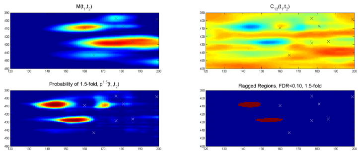
Specific Results 2: Posterior mean of overall mean gel (upper left), effect gel (upper right), probability discovery plot (lower left), and indicating WFMM flagged regions (lower right) for region marked by large box in Figure 4, with pinnacles for detected spots marked (x), and differential expression in Pinnacle analysis indicated by a (o). Note that regions flagged by WFMM correspond to tails of visible spots that themselves are not differentially expressed. These results are not found by the Pinnacle analysis. Reproduced with permission from The Annals of Applied Statistics [45]

5.5 Extensions

There is great potential for further methodological development of the functional mixed model framework beyond the WFMM presented in Section 5. We will briefly summarize two valuable extensions of the WFMM: one that leads to robust modeling and inference and one that extends the approach to other basis functions and transformations.

Robust Functional Mixed Models (RWFMM)

The FMM underlying the WFMM allows one to perform multiple regression of functional responses on a variety of predictors. While allowing flexible, nonparametric forms for the fixed effect functions, which are the functional regression coefficients, the estimation and inference are sensitive to outlying curves and regions of curves because of the Gaussian assumptions underlying the model. To produce robust functional regression, we developed a new multi level hierarchical model for the WFMM framework with separate scale parameters for each curve and each wavelet coefficient at different levels of modeling: fixed effects, random effects, and residual errors [70]. Conditional on these scale parameters, the model is Gaussian, so we can use the efficient code and analytical tractability of the Gaussian WFMM, but integrating out these parameters we are left with heavier-tailed distributions.

These heavy-tailed distributions for the residual errors cause the functional regression to be a weighted functional regression in the wavelet space, with outlying observations for each wavelet coefficient downweighted in estimation of the fixed and random effects. The heavy-tailed distributions for the random effects similarly lead to a downweighting of outlying random effect units in estimation and inference of the functional fixed effects. As a result, we are left with robust estimation and inference for the random and fixed effect functions. It can be shown that, with this modeling framework, as an entire curve or part of a curve goes to infinity, the influence of the diverging data goes to zero, and the posterior distribution conditions only on the non-diverging parts of the curves [70]. In simulation studies based on the pancreatic cancer MALDI-TOF data set described in Section 2 [70], we demonstrate that for heavier-tailed random effects and residuals, the robust WFMM dominates the Gaussian WFMM; when the data are in fact Gaussian, there is a less than 10% loss of efficiency in using the robust model. This robustness property leads to considerably improved classification results [71], since the WFMM-based classification can be sensitive to outlying curves and wavelet coefficients (see Table 1).

Also, this hierarchical model underlying the robust WFMM induces prior distributions on the random effect functions and fixed effect functions that have better sparsity and variable selection properties than the Gaussian and spike-Gaussian slab priors used in the GWFMM. The induced distributions have connections to the adaptive lasso [72] and the normal-exponential-gamma (NEG) prior distribution [30]. When applied in the wavelet space, these priors can lead to more effective adaptive regularization, thus allowing the model to do a better job of removing spurious features of the fixed and random effect functions while retaining true local features, as demonstrated by the simulation study [70]. This improved adaptive smoothing may partially explain our results that the RWFMM analysis led to more flagged spectral regions than the GWFMM analysis when applied to a MALDI-TOF example [70].

Beyond Wavelets: Isomorphic Functional Mixed Models with other Basis Functions

Wavelets are a compelling choice of basis representation for irregular functional data, and appear to work well for many different types of functional data. The FMM can be fit using the same 3-step approach underlying the WFMM but using other basis functions, or more generally using some invertible transformation of the observed functions [45]. The key idea of this multi domain modeling approach is that we transform the data into an alternative domain where modeling can be done more parsimoniously and effectively, and we then transform results back to the original data domain for inference and interpretation. It is especially appealing to use what we term an isomorphic transformation, which is one that preserves all of the information in the original data (i.e., is invertible or lossless). More precisely, given row vector y ∈ ( ), we say a transform f: ( ) → ( ) is isomorphic if there exists a reverse transform f⁻¹ such that f⁻¹{f(y)} = y. The wavelet transform is isomorphic because IDWT(DWT(y))= y, but isomorphic transformations can be constructed in other ways as well, for example, by using other basis functions including Fourier bases, spline bases, and certain empirically determined basis functions like functional principal components, or even nonlinear transformations. Given a choice of transformation, one must carefully consider the implications of the distributional and covariance assumptions made in the alternative transformed domain in the data space model to ensure that the modeling approach makes sense.

6. DISCUSSION AND CONCLUSIONS

Proteomics is an exciting, growing field with many challenges ahead. Undoubtedly, new proteomic technologies and approaches that help overcome some of the current limitations will emerge. Moving forward, it will remain important to give careful consideration to statistical issues, including experimental design, preprocessing, and analysis, if the field is going to reach its potential in detecting useful proteomic markers.

Experimental design is a crucial but underappreciated aspect of proteomic studies. It is important to think carefully about issues like batch effects and to prospectively incorporate design principles such as blocking and randomization to ensure that nuisance factors are not confounded with factors of interest, thus preventing effective comparative proteomics studies. Effective preprocessing must be done to get the proteomic spectra and images ready for analysis.

Feature extraction remains the dominant mode of analysis for proteomic data. It is efficient and can be effective, as long as the feature extraction approaches used are sensitive and precise. This is crucial, since subsequent analyses, whether group comparison, classification, or unsupervised clustering, conditions on these determinations. An emerging alternative is to use flexible functional data analysis modeling techniques to model the proteomic spectra or images and perform analysis, which does not depend on feature extraction. This approach promises to find discoveries that could be missed by the feature extraction approach because of co-migrating proteins, but any effective approach must be flexible enough to capture the complex local features characterizing these data and must be computationally efficient enough to handle these studies’ large sample sizes. The wavelet-based functional mixed model [47] appears to be an effective approach for these data. The approach scales up to higher dimensional data like images, to other basis functions, and to robust analyses. Further study and software interface development are necessary to get these methods more accessible to proteomic investigators.

Statistics and other quantitative sciences will need to continue to make a strong contribution for proteomics to reach its full potential.

References

- 1.Aebersold R, Mann M. Mass spectrometry-based proteomics. Nature. 2003;422:198–207. doi: 10.1038/nature01511. [DOI] [PubMed] [Google Scholar]
- 2.Ahmed SH, Koob GF. Transition from moderate to excessive drug intake: change in hedonic set point. Science. 1998;282(5387):298–300. doi: 10.1126/science.282.5387.298. [DOI] [PubMed] [Google Scholar]
- 3.Ahn J, Marron JS, Muller KM, Chi YY. The high-dimension, low-sample-size geometric representation holds under mild conditions. Biometrika. 2007;94:760–766. [Google Scholar]
- 4.Baggerly KA, Coombes KR, Morris JS. Bias, randomization, and overian proteomic data. Cancer Informatics. 2005;1(1):9–14. [PMC free article] [PubMed] [Google Scholar]
- 5.Baggerly KA, Edmonson S, Morris JS, Coombes KR. High-resolution serum proteomic patterns for ovarian cancer detection. Endocrine-Related Cancers. 2004;11(4):583–584. doi: 10.1677/erc.1.00868. [DOI] [PubMed] [Google Scholar]
- 6.Baggerly KA, Morris JS, Coombes KR. Reproducibility of seldi mass spectrometry patterns in serum: Comparing proteomic data sets from different experiments. Bioinformatics. 2004;20(5):777–785. doi: 10.1093/bioinformatics/btg484. [DOI] [PubMed] [Google Scholar]
- 7.Baggerly KA, Morris JS, Edmonson S, Coombes KR. Reproducibility of selditof protein patterns in serum: comparing datasets from different experiments. Journal of the National Cancer Institute. 2005;97:307–309. [Google Scholar]
- 8.Baik J, Ben Arous G, Peche S. Phase transition of the largest eigenvalue for nonnull complex sample covariance matrices. Annals of Probablity. 2005;33:1643–1697. [Google Scholar]
- 9.Baik J, silverstein JW. Eigenvalues of large sample covariance matrices of spiked population models. Journal of Multivariate Analysis. 2006;97:1382–1408. [Google Scholar]
- 10.Benjamini Y, Hochberg Y. Controlling the false discovery rate: a practical and powerful approach to multiple testing. JRSS-B. 1995;57:289–300. [Google Scholar]
- 11.Benjamini Y, Liu W. A step-down multiple hypotheses testing procedure that controls the false discovery rate under independence. Journal of Statistical Planning and Inference. 1999;82:163–170. [Google Scholar]
- 12.Bondell HD, Reich BJ. Simultaneous regression shrinkage, variable selection, and supervised clustering of predictors with oscar. Biometrics. 2008;64:115–123. doi: 10.1111/j.1541-0420.2007.00843.x. [DOI] [PMC free article] [PubMed] [Google Scholar]
- 13.Carvalho CM, Polson NG, Scott JG. The horseshoe estimator for sparse signals. Biometrika. 2010;97(2):465–480. [Google Scholar]
- 14.Chen J, Sarkar SK. A bayesian determination of threshold for identifying differentially expressed genes in microarray experiments. Statistics in Medicine. 2006;25:3174–3189. doi: 10.1002/sim.2422. [DOI] [PubMed] [Google Scholar]
- 15.Clark BN, Gutstein HB. The myth of automated, high-throughput two-dimensional gel analysis. Proteomics. 2008;8:1197–1203. doi: 10.1002/pmic.200700709. [DOI] [PubMed] [Google Scholar]
- 16.Conrads TP, Fusaro VA, Ross S, Johann D, Rajapakse V, Hitt BA, Steinberg SM, Kohn EC, Fishman DA, Whitely G, Barrett JC, Liotta LA, Petricoin EF, Veenstra TD. High-resolution serum proteomic features of ovarian cancer detection. Endocrine Related Cancer. 2004;11(2):163–178. doi: 10.1677/erc.0.0110163. [DOI] [PubMed] [Google Scholar]
- 17.Coombes KR, Tsavachidis S, Morris JS, Baggerly KA, Hung MC, Kuerer HM. Improved peak detection and quantification of mass spectrometry data acquired from surface-enhanced laser desorption and ionization by denoising spectra with the undecimated discrete wavelet transform. Proteomics. 2005;5:4107–4117. doi: 10.1002/pmic.200401261. [DOI] [PubMed] [Google Scholar]
- 18.Crainiceanu CM, Staicu AM, Di C. Generalized multilevel functional regression. Journal of the American Statistical Association. 2009;104(488):1550–1561. doi: 10.1198/jasa.2009.tm08564. [DOI] [PMC free article] [PubMed] [Google Scholar]
- 19.Datta S, Datta S. Empirical bayes screening of many p-values with applications to microarray studies. Bioinformatics. 2005;21(9):1987–1994. doi: 10.1093/bioinformatics/bti301. [DOI] [PubMed] [Google Scholar]
- 20.Deutsch EW, Lam H, Aebersold R. Data analysis and bioinformatics tools for tandem mass spectrometry in proteomics. Physiol Genomics. 2008;33(1):18–25. doi: 10.1152/physiolgenomics.00298.2007. [DOI] [PubMed] [Google Scholar]
- 21.Dowsey A, Dunn M, Yang G. Automated image alignment for 2d gel electrophoresis in a high-throughput proteomics pipeline. Bioinformatics. 2008;24:950–957. doi: 10.1093/bioinformatics/btn059. [DOI] [PubMed] [Google Scholar]
- 22.Dowsey AW, English JA, Lisacek F, Morris JS, Yang GZ, Dunn MJ. Advance article a22975: Image analysis tools in proteomics. Encyclopedia of Life Sciences. 2010 doi: 10.1002/pmic.200900635. [DOI] [PMC free article] [PubMed] [Google Scholar]
- 23.Dowsey AW, English JA, Lisacek F, Morris JS, Yang GZ, Dunn MJ. Image analysis tools and emerging algorithms for expression proteomics. Proteomics. 2010;10(23):4226–4257. doi: 10.1002/pmic.200900635. [DOI] [PMC free article] [PubMed] [Google Scholar]
- 24.Dowsey AW, Morris JS, Gutstein HG, Yang GZ. Informatics and statistics for analyzing 2-d gel electrophoresis images. Methods in Molecular Biology. 2010;604:239–255. doi: 10.1007/978-1-60761-444-9_16. [DOI] [PMC free article] [PubMed] [Google Scholar]
- 25.Dubitzky W, Granzow M, Berrar D. Fundamentals of Data Mining in Genomics and Proteomics. Kluwer; Boston: 2007. [Google Scholar]
- 26.Efron B. Large-scale simultaneous hypothesis testing: the choice of a null hypothesis. Journal of the American Statistical Association. 2004;99:96–104. [Google Scholar]
- 27.Fan J, Li R. Variable selection via nonconcave penalized likelihood and its oracle properties. JASA. 2001;96(456):1348–1360. [Google Scholar]
- 28.Fenn JB, Mann M, Meng CK, Wong SF, White-house CM. Electrospray ionization for mass spectrometry of large biomolecules. Science. 1989;246(4926):64–71. doi: 10.1126/science.2675315. [DOI] [PubMed] [Google Scholar]
- 29.Genovese C, Wasserman L. Operating characteristics and extensions of the false discovery rate procedure. JRSS-B. 2002;64:499–517. [Google Scholar]
- 30.Griffin JE, Brown PJ. CRiSM Working Paper No 05–10. University of Warwick; 2005. Alternative prior distributions for variable selection with very many more variables than observations. http://www.cs.berkeley.edu/russell/classes/cs294/f05/papers/griffin+brown-2005.pdf. [Google Scholar]
- 31.Gygi SP, Corthals GL, Zhang Y, Rochon Y, Aebersold R. Evaluation of two-dimensional gel electrophoresis-based proteome analysis technology. Proceedings of the National Academy of Sciences of the United States of America. 2000;97(17):9390–9395. doi: 10.1073/pnas.160270797. [DOI] [PMC free article] [PubMed] [Google Scholar]
- 32.Hall P, Marron JS, Neeman A. Geometric representation of high dimension, low sample size data. JRSS-B. 2005;67:427–444. [Google Scholar]
- 33.Herrick RC, Morris JS. Wavelet-based functional mixed model analysis:computational considerations. Proceedings, Joint Statistical Meetings, ASA Section on Statistical Computing; 2006. pp. 2051–2053. [Google Scholar]
- 34.Hu J, Coombes KR, Morris JS, Baggerly KA. The importance of experimental design in proteomic mass spectrometry experiments: Some cautionary tales. Briefings in Functional Genomics and Proteomics. 2005;3(4):322–331. doi: 10.1093/bfgp/3.4.322. [DOI] [PubMed] [Google Scholar]
- 35.Ishwaran H, Rao JS. Detecting differentially expressed genes in microarrays using bayesian model selection. Journal of the American Statistical Association. 2003;98:438–455. [Google Scholar]
- 36.Johnstone I. On the distribution of the largest eigenvalue in principal component analysis. Annals of Statistics. 2001;29:295–327. [Google Scholar]
- 37.Jung S, Marron JS. Pca consistency in high dimension, low sample size context. The Annals of Statistics. 2009;37(6B):4104–4130. [Google Scholar]
- 38.Karas M, Bachman D, Bahr U, Hillencamp F. Matrix assisted ultraviolet laser desorption of non-volatile compounds. International Journal of Mass Spectrometry and Ion Physics. 1987;78:53–68. [Google Scholar]
- 39.Karp NA, Lilley KS. Maximizing sensitivity for detecting changes in protein expression: Experimental design using minimal cydyes. Proteomics. 2005;5:3105–3115. doi: 10.1002/pmic.200500083. [DOI] [PubMed] [Google Scholar]
- 40.Karpievitch YV, Hill EG, Morris JS, Coombes KR, Baggerly KA, Almeida JS. Prepms: Tof ms data graphical preprocessing tool. Bioinformatics. 2007;23(2):264–265. doi: 10.1093/bioinformatics/btl583. [DOI] [PMC free article] [PubMed] [Google Scholar]
- 41.Koomen JM, Shih LN, Coombes KR, Li D, Xiao LC, Fidler IJ, Abbruzzese JL, Kobayashi R. Plasma protein profiling for diagnosis of pancreatic cancer reveals the presence of host response proteins. Clinical Cancer Research. 2005;11(3):1110–1118. [PubMed] [Google Scholar]
- 42.Leek JT, Storey JD. A general framework for multiple testing dependence. PNAS. 2008;105(48):18718–18723. doi: 10.1073/pnas.0808709105. [DOI] [PMC free article] [PubMed] [Google Scholar]
- 43.Mallat S. A theory for multiresolution signal decomposition: the wavelet representation. IEEE Transactions on Pattern Analysis and Machine Intelligence. 1989;11:674–693. [Google Scholar]
- 44.Morris JS, Baggerly KA, Gutstein HB, Coombes KR. Statistical contributions to proteomic research. Methods in Molecular Biology. 2010;641:143–166. doi: 10.1007/978-1-60761-711-2_9. [DOI] [PMC free article] [PubMed] [Google Scholar]
- 45.Morris JS, Baladandayuthapani V, Herrick RC, Sanna P, Gutstein H. Automated analysis of quantitative image data using isomorphic functional mixed models, with application to proteomics data. Annals of Applied Statistics. 2011;5(2A):894–923. doi: 10.1214/10-aoas407. [DOI] [PMC free article] [PubMed] [Google Scholar]
- 46.Morris JS, Brown P, Herrick R, Baggerly K, Coombes K. Bayesian analysis of mass spectrometry data using wavelet-based functional mixed models. Biometrics. 2008;12:479–489. doi: 10.1111/j.1541-0420.2007.00895.x. [DOI] [PMC free article] [PubMed] [Google Scholar]
- 47.Morris JS, Carroll RJ. Wavelet-based functional mixed models. Journal of the Royal Statistical Society, B. 2006;68(2):179–199. doi: 10.1111/j.1467-9868.2006.00539.x. [DOI] [PMC free article] [PubMed] [Google Scholar]
- 48.Morris JS, Clark B, Gutstein H. Pinnacle: A fast, automatic and accurate method for detecting and quantifying protein spots in 2-dimensional gel electrophoresis data. Bioinformatics. 2008;24:529–536. doi: 10.1093/bioinformatics/btm590. [DOI] [PMC free article] [PubMed] [Google Scholar]
- 49.Morris JS, Clark BN, Wei W, Gutstein HB. Evaluating the performance of new approaches to spot quantification and differential expression in 2-dimensional gel electrophoresis studies. Journal of Proteome Research. 2010;9(1):595–604. doi: 10.1021/pr9005603. [DOI] [PMC free article] [PubMed] [Google Scholar]
- 50.Morris JS, Coombes K, Kooman J, Baggerly K, Kobayashi R. Feature extraction and quantification for mass spectrometry data in biomedical applications using the mean spectrum. Bioinformatics. 2005;21:1764–1775. doi: 10.1093/bioinformatics/bti254. [DOI] [PubMed] [Google Scholar]
- 51.Morris JS, Vannucci M, Brown PJ, Carroll RJ. Wavelet-based nonparametric modeling of hierarchical functions in colon carcinogenesis. Journal of the American Statistical Association. 2003;98(463):573–583. with discussion. [Google Scholar]
- 52.Mueller LN, Brusniak MY, Mani DR, Aebersold R. An assessment of software solutions for the analysis of mass spectrometry based quantitative proteomics data. Journal of Proteome Research. 2008;7(1):51–61. doi: 10.1021/pr700758r. [DOI] [PubMed] [Google Scholar]
- 53.Newton MA, Noueiry A, Sarkar D, Ahlquist P. Detecting differential gene expression with a semiparametric hierarchical mixture method. Biostatistics. 2004;5(2):155–176. doi: 10.1093/biostatistics/5.2.155. [DOI] [PubMed] [Google Scholar]
- 54.O’Farrell PH. High-resolution two-dimensional electrophoresis of proteins. J Biol Chem. 1975;250:4007–4021. [PMC free article] [PubMed] [Google Scholar]
- 55.Ogden RT. Essential Wavelets for Statistical Applications and Data Analysis. Birkhäuser; Boston, USA: 1997. [Google Scholar]
- 56.O’Hara RB, Sillanpaa MJ. A review of bayesian variable selection methods: What, how and which. Bayesian Analysis. 2009;4(1):85–118. [Google Scholar]
- 57.Parsons LH, Koob GF, Weiss F. Serotonin dysfunction in the nucleus accumbens of rats during withdrawal after unlimited access to intravenous cocaine. Journal of Pharmacology and Experimental Therapeutics. 1995;274:1182–1191. [PubMed] [Google Scholar]
- 58.Paul D. Asymptotics of sample eigenstructure for a large dimensional spiked covariance model. Statistical Sinica. 2007;17:1617–1642. [Google Scholar]
- 59.Pounds S, Cheng C. Improving false discovery rate estimation. Bioinformatics. 2004;20(11):1737–1745. doi: 10.1093/bioinformatics/bth160. [DOI] [PubMed] [Google Scholar]
- 60.Pounds S, Morris SW. Estimating the occurrence of false positives and false negatives in microarray studies by approximating and partitioning the empirical distribution of p-values. Bioinformatics. 2003;19(10):1236–1242. doi: 10.1093/bioinformatics/btg148. [DOI] [PubMed] [Google Scholar]
- 61.Ramsay JO, Silverman BW. Functional Data Analysis. Springer-Verlag; New York: 2006. [Google Scholar]
- 62.Sherman NE, Kinter M. Protein sequencing and identification using tandem mass spectrometry. Wiley; New York: 2000. [Google Scholar]
- 63.Storey JD. A direct approach to false discovery rates. JRSS-B. 2002;64:479–498. [Google Scholar]
- 64.Storey JD. The positive false discovery rate: a bayesian interpretation and the q-value. The Annals of Statistics. 2003;31:2013–2035. [Google Scholar]
- 65.Strimmer K. A unified approach to false discovery rate estimation. BMC Bioinformatics. 2008;9:303. doi: 10.1186/1471-2105-9-303. [DOI] [PMC free article] [PubMed] [Google Scholar]
- 66.Tibshirani RJ. Regression shrinkage and selection via the lasso. JRSS-B. 1996;58:267–288. [Google Scholar]
- 67.Twyman RM. Principles of Proteomics. Bios Scientific Publishers, Taylor & Francis Groups; Independence, KY: 2004. [Google Scholar]
- 68.Vidakovic B. Statistical Modeling by Wavelets. John Wiley & Sons; Chichester, England: 1999. [Google Scholar]
- 69.Yekutielli D, Benjamini Y. Resampling-based false discovery rate controlling multiple test procedures for correlated test statistics. Journal of Statistical Planning and Inference. 1999;82:171–196. [Google Scholar]
- 70.Zhu H, Brown PJ, Morris JS. Robust, adaptive functional regression in functional mixed model framework. JASA. 2011;106(495) doi: 10.1198/jasa.2011.tm10370. [DOI] [PMC free article] [PubMed] [Google Scholar]
- 71.Zhu H, Brown PJ, Morris JS. Robust classification of functional and quantitative image data using functional mixed models. Biometrics. doi: 10.1111/j.1541-0420.2012.01765.x. to appear, 2012. [DOI] [PMC free article] [PubMed] [Google Scholar]
- 72.Zou H. The adaptive lasso and its oracle properties. JASA. 2006;101:1418–1429. [Google Scholar]