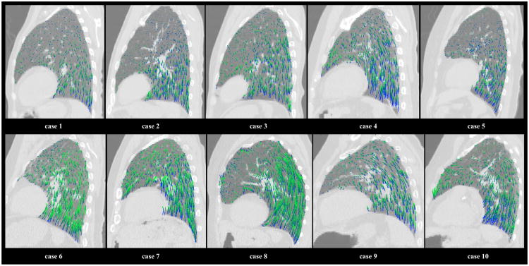
Figure 7. Calculated temporal motion sequences.

For each reference case, an example T00 sagittal view is shown with a random sample of the corresponding in-plane trajectories calculated using the cubic 4DLTM algorithm. The plotted trajectories are color-coded to indicate their temporal sequence. The initial T00 →T10 displacements are shown in blue, while each subsequent displacement gradually changes shade towards dark green. The calculated motion sequences are seen to vary widely across the 10 reference cases, both in time and space. The corresponding quantitative error assessment for each case is shown in Table 4.