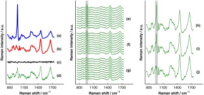
Fig. 4.

Example of simulated data set used to compare the performances of SOLD and BTEM. The (a) bone and (b) soft-tissue spectra were generated from the spectra in Fig. 3. A spectrum of zero-mean, Gaussian noise (c) was added to a linear combination of the bone and soft-tissue spectra to form a single transcutaneous spectrum (d). This process was repeated to generate 30 transcutaneous spectra [(e), (f), and (g)] with varying contributions of the bone and soft-tissue spectra. These 30 spectra represent a transcutaneous data set acquired from a single measurement site. The set of 30 spectra was submitted to BTEM to estimate the underlying spectrum of bone. In addition, each set of 10 spectra grouped together in (e), in (f), and in (g) was summed, yielding three spectra [(h), (i), and (j)] that were submitted to SOLD. The entire process summarized in this figure was repeated 100 times (with different pairs of underlying bone and soft-tissue spectra) to simulate transcutaneous data acquired from different samples. The gray bars highlight the ${\mathrm{PO}}_4^{3-}$ ${\nu }_1$ peak, which is present in the spectrum of bone. The amplitude of this peak qualitatively represents the contribution of bone to each transcutaneous spectrum.