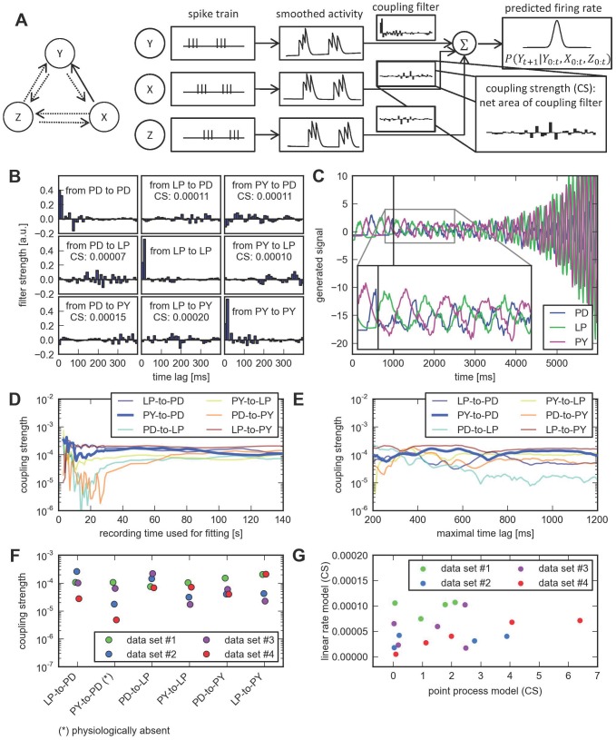
Figure 4. A linear firing rate model is insufficient to reconstruct the correct connectivity.
A, Schematic overview of the linear rate model. First, spike trains are convolved with a smoothing filter to obtain smoothed time series of firing rates for all neurons (here denoted by X, Y and Z). Linear models are estimated for each neuron (Y) by including auto- and cross-regressive terms from the filtered input of putatively presynaptic neurons (here, X and Z). The firing rate is assumed to be Gaussian with the linearly predicted mean and fixed standard deviation. B, Estimated interactions. Coupling coefficients for the auto- (diagonal) and cross-regressive terms (off-diagonal) of the linear model are shown. The maximal time lag was chosen to be 400 ms to match the model of Kispersky et al. [29]. Coupling strength is defined as the net area under the interaction kernel. C, The linear rate model fails to generate pyloric-like activity. Neural activity was simulated from the fitted model. First, model output was clamped to the observed activity traces for one second (vertical line). Subsequent activity was simulated using the predictions of the model and a stochastic realization of the noise term. The triphasic burst rhythm is not maintained and modeled neural firing rates diverge after a few seconds of simulated time. D–E, The linear model does not accurately reproduce the known physiological connectivity for a wide range of parameter choices, such as the length of the data set (D) or a maximal time lag different from 400 ms (E). F, Network inference using the linear model for all four data sets. The physiologically nonexistent connection corresponds to the weakest one in only two out of the four cases. Horizontal scatter is for visualization only. G, Coupling strengths (CS) for the point process model (horizontal axis) and linear rate model (vertical axis) are uncorrelated. The scatter plot shows the six cross-couplings for each of the four data sets. The coupling strength for the two models are not significantly correlated ( ,
,  ).
).

