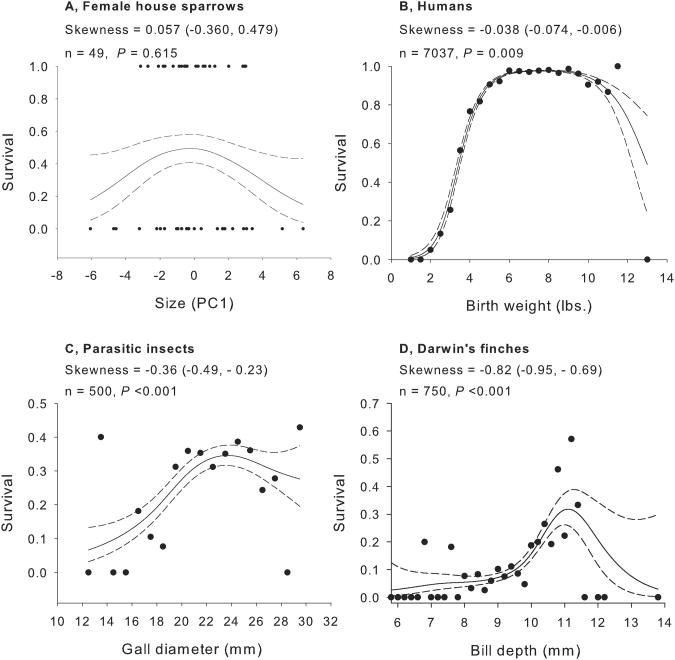
Fig. 1. Iconic examples of stabilizing selection.

Examples are arranged in order of increasingly negative skewness, where the left tail is flatter, including a) survival of house sparrows ³³ based on body size, b) human baby survival based on birth weight ¹⁴, c) survival of the parasitic insect Eurosta solidaginis from 1984-5 based on gall diameter ¹⁵, and d) survival of Darwin's finches (Geospiza spp.) on Daphne Island from 1976-1978(including immigrant birds)based on bill depth ¹⁶. Lines indicate the best cubic spline fit (± 1 SEM) as per Schluter⁸. For presentation, we bin survival data in large datasets and depict average survival. To calculate skewness, we first estimated predicted values for 200 equally spaced points across the range of trait values to discretize the smoothed fitness surface to avoid giving undue weight to outliers. We then calculated 10,000 estimates of skewness using the original number of samples with replacement and with probability equal to relative fitness. We calculated 95% confidence intervals around mean skewness and the probability that skewness was zero or opposite in sign from estimated mean skewness.