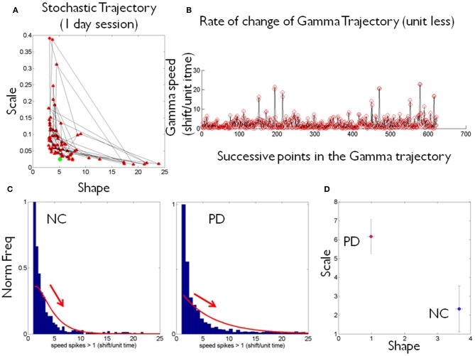
Figure 2.

Schematics to illustrate the second step in the methods using data from one patient and one control. (A) Shows an example of a stochastic trajectory of a PD participant on the Gamma plane for 1 day. The green dot marks the start of the trajectory. (B) The change in position of the point (unit less) along the stochastic trajectory was obtained over time. This is the change in the Euclidean distance in the Gamma plane between two successive points. Each point in the trajectory on the Gamma plane is estimated using at least 100 point measurements (one data entry) of many in a recording session, across several sessions within a given day. (C) Sample histograms of the speed spikes >1 (in shifts/unit time) for 1 day plotted for a NC and a PD participant. The histograms and bin size estimation for the parameters of interest were obtained using MATLAB routines developed in-house based on well-established algorithms for optimal estimation with W = 3.49σN^−1/3 (Izenman, 1991), where W is the bin width, σ the standard deviation of the distribution (we used estimated standard deviation $\widehat{\sigma }$) and N the number of samples. Arrows show the exponential decay in each case. (D) Example of estimated (shape, scale) point for each of the NC and PD cases in (C) are plotted on the Gamma plane with 95% confidence intervals.