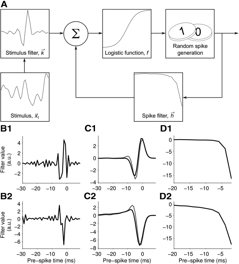
Figure 4.

Model structure and parameter fitting. A, Schematic of the GLM. The linear filters k⃗ and h⃗ are convolved with the whisker stimulus and spike history, respectively. The resulting coefficients are summed with the constant b and passed through the nonlinear function f(·) to produce the time-dependent probability of a spike. B1, Stimulus filter for an example unit. C1, The stimulus filter convolved with the white noise autocorrelation (black line), compared with the unit's STA (gray line). D1, The unit's spike feedback filter. B2–D2, Corresponding results for a second example unit.