Figure 2. Schematic of LN and NIM structures.

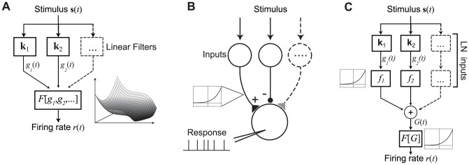
A) Schematic diagram of an LN model, with multiple filters (k₁, k₂, …) that define the linear stimulus subspace. The outputs of these linear filters (g ₁, g ₂, …) are then transformed into a firing rate prediction r(t) by the static nonlinear function F[g ₁,g ₂,…], depicted at right for a two-dimensional subspace. Note that while the general LN model thus allows for a nonlinear dependence on multiple stimulus dimensions, estimation of the function F[.] is typically only feasible for low (one- or two-) dimensional subspaces. B) Schematic illustration of a generic neuron that receives input from a set of ‘upstream’ neurons that are themselves driven by the stimulus s. Each of the upstream neurons provides input to the model neuron that is generally rectified due to spike generation (inset at left), and thus is either excitatory or inhibitory. The model neuron then integrates its inputs and produces a spiking output. C) Block diagram illustrating the structure of the NIM, based on (B). The set of inputs are represented as (one-dimensional) LN models, with a corresponding stimulus filter k_i, and “upstream nonlinearity” f_i(.). These inputs are then linearly combined, with weights w _i, and fed into the spiking nonlinearity F[.], resulting in the predicted firing rate r(t). The NIM thus has a ‘second-order LN’ structure (or LNLN), with the neuron's own nonlinear processing shaped by the LN nature of its inputs.