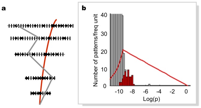
Figure 2. Monte Carlo simulation of track reconstruction and pattern filtering in a HEP particle detector.

a, Schematic representation of a sector of a four-layers tracking detector, with simulated data (see Methods). Black dots represent measured positions where flying particles cross the detector layers - they can also be produced by random noise. Each layer is subdivided into a finite number of intervals (bins), delimited here by vertical bars. Every possible combination of bins (one on each layer) defines a pattern (grey line example). Only a small fraction of the patterns are compatible with the presence of a real particle (red line example), b, Probability distribution of the frequency of patterns (δ(p)) produced by a sample of simulated events of the type shown in (a) (grey histogram). The distribution of the sub-sample of patterns corresponding to valid particle trajectories is shown as a red histogram. The red curve is the function of eq. 1, with N = 50 and W = 0.15. The vertical red lines indicate the probability range selected by our model, using the constraint ∫_f(p)>c pδ(p)dp<W.