
Figure 3. Power of length and joint tests corresponds to the behavior predicted by geometric framework.
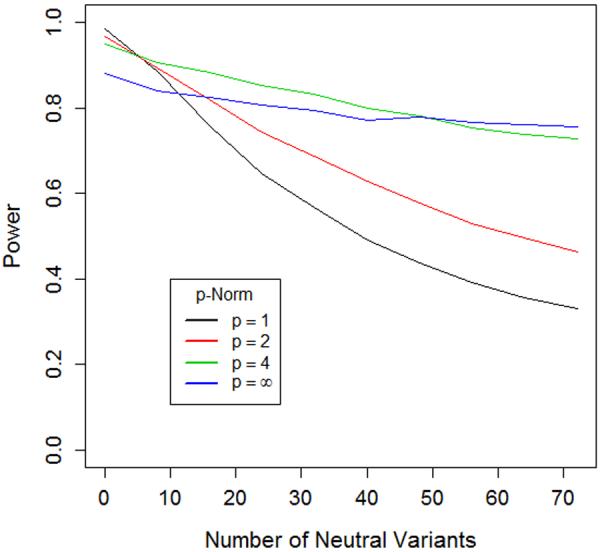
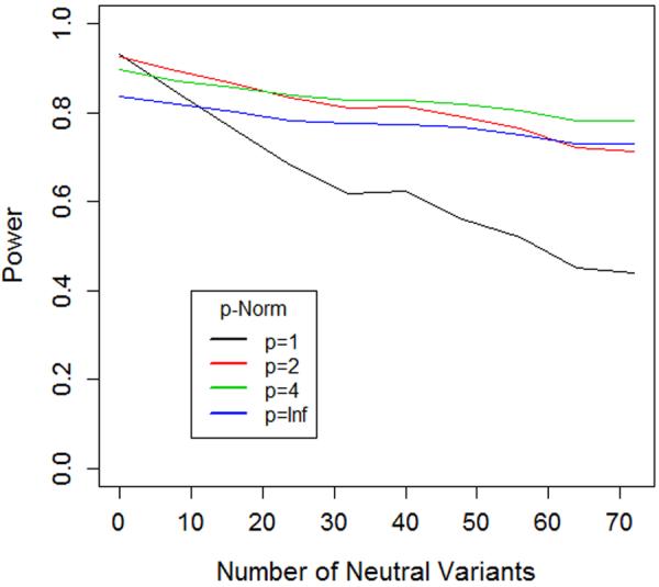
The two graphs illustrate the power of length (Lp = ∥f+∥p − ∥f−∥p)and joint tests (Jp = ∥f+ − f−∥p) with different norms (p=1, 2, 4 and ∞). In each case the test statistic is computed and significance is assessed via permutation of case-control status. We consider a scenario where a gene contains eight causal risk variants, all with a relative risk of 2.0. Two of the risk variants have MAF=1%, the other six have MAF=0.1%. We simulated a sample of 1000 cases and 1000 controls for this setting. We then considered 9 additional settings where we added 8, 16, 24, 32, 40, 48, 56, 64 and 72 additional non-causal variants (relative risk=1), always maintaining 3:1 ratio of low MAF (0.1%) to high MAF (1%) variants in the set.
A) For Lp, as we move from no non-causal variants to 72 non-causal variants, the order of most powerful tests completely reverses, suggesting that higher norms are more optimal in situations with large numbers of non-causal variants.
B) For Lp, as we move from no non-causal variants to 72 non-causal variants, the order of most powerful tests nearly reverses, suggesting that, once again, higher norms are more optimal in situations with large numbers of non-causal variants.