Figure 1.

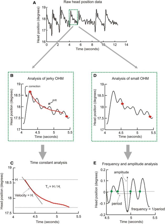
Schematic for data analysis. A depicts typical raw head position data from a CD patient. The head position waveform had high amplitude jerky head oscillations and superimposed small sinusoidal oscillations. The first step was to interactively select a region of interest (green box in A). To analyze the large jerky oscillatory head movements, we identified drift of the head position in the region of interest between two red dots (B). The signal was then subject to a Savitzsky–Golay filter, and the time constant of drift in filtered head position was computed (C). To analyze the smaller sinusoidal oscillatory movements, the region of interest between two red dots (D) within the region of interest in the green box (A) was interactively selected and detrended (E). Time points of intersection of zero-line and the signal moving from negative to positive were determined. The difference of these time points was considered as period of oscillation, and the oscillation frequency was determined as the inverse of the time period. H, Initial head position; Hi, Initial head velocity; Tc, decay time constant; OHM, oscillatory head movements.