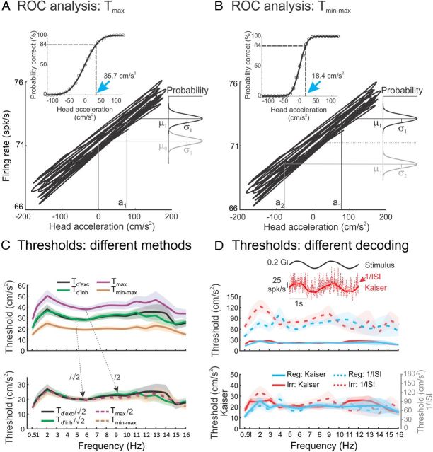
Figure 4.

Comparison between neural thresholds obtained using different methodologies for otolith afferents. A, B, Plots of the instantaneous firing rate as a function of linear acceleration for the same example regular afferent. We compared the firing rate distributions for a given positive value of acceleration Ḧ (black Gaussian curves) and that obtained for zero linear acceleration (i.e., Ḧ = 0) (gray curve in A) or the firing rate distribution when the acceleration has the opposite value (i.e., −Ḧ) (gray curve in B). The insets illustrate the corresponding neurometric functions obtained using ROC analysis. The detection T_max and discrimination T_min−max thresholds were computed as the values of linear acceleration for which the probability of correct detection is equal to 84% (blue arrows in A and B, respectively). C, Top, Population-averaged neural threshold values computed using different methodologies: T_d′exc (black) and T_d′inh (green) were computed using d′ as described in Figure 3 but using only positive or negative values of head acceleration, respectively. T_max (purple) and T_min−max (orange) are also shown for comparison. Bottom, Same measures but normalized such that both T_d′exc and T_d′inh are divided by $\sqrt{2}$ and T_max is divided by 2. It is seen that all curves then coincide (ANOVA, p > 0.54 for all stimulus frequencies), which illustrates that the different methodologies used to compute neural thresholds lead to estimates that differ only by a proportionality constant that is independent of frequency. D, Top, Population-averaged T_min−max values for regular (blue, Reg) and irregular (red, Irr) afferents obtained when the firing rate is estimated using the inverse ISI (dashed) and a Kaiser filter (solid). It is seen that using a Kaiser filter gives rise to significantly lower threshold estimates (t test, p < 0.05 for all frequencies). However, both regular and irregular afferents display thresholds that are not significantly different from one another using either methodology (t test, Kaiser filter, p > 0.05 for all frequencies; 1/ISI, p > 0.05 for all frequencies). The inset illustrates the firing rates estimated by the reciprocal ISI (dashed red) and Kaiser filter (solid red) to a 0.5 Hz sinusoidal head acceleration stimulus (solid black). Bottom, Same quantities as a function of stimulus frequency using a double y-axis plot. The fact that all curves superimpose illustrates that using different methodologies to estimate firing rate will give rise to threshold estimates that only differ by a proportionality constant that is independent of frequency. We found empirically that dividing the threshold values estimated from the inverse ISI by 3.6 gave rise to values that were not significantly different from those obtained using the Kaiser filter (t test, p > 0.13 and p > 0.07 for regular and irregular afferents, respectively, for every stimulus frequency). The shaded bands represent 1 SEM.