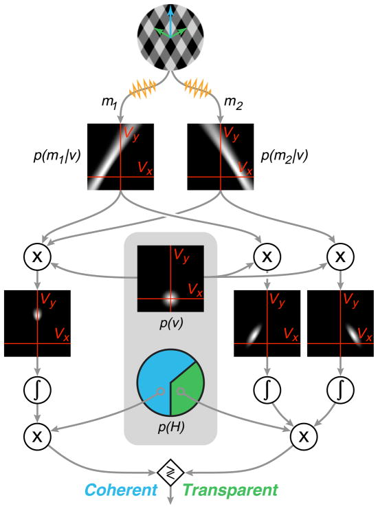
Figure 2.

Illustration of the Bayesian observer model, responding to a single presentation of a plaid. In the encoding stage (not shown), an observer makes noisy measurements {m⃑₁, m⃑₂} of the normal velocities of the two gratings. In the decoding stage, the observer forms separate likelihood functions for the two component motions based on their associated measurements. These are combined with prior preferences (internal to the observer’s visual system) in order to arrive at a percept. Internal preferences are contained within the gray region and include a prior distribution over velocity, p(v⃑), and a prior probability of coherent motion, p(H). For the coherent motion percept, both likelihoods are multiplied together with the velocity prior, and this posterior distribution is then integrated (left). For the transparent percept, each likelihood is individually multiplied by the velocity prior and integrated (right). The resulting scalar values are then multiplied by the internal prior for coherence/transparency, yielding posterior probabilities for each of the percepts. Finally, these are compared, and the larger one is selected as the percept.