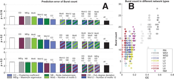
Figure 6. Burst count is best predicted using CC when in-degree is binomial.

A: The bars in the three panels show the prediction errors (mean + std, ) when different graph properties are used as predictors. The errors are calculated as the difference between the predicted and realized number of bursts. The HH model is used in purely excitatory networks with binomial in-degree distribution and average connectivities (upper), (middle) and (lower). The leftmost bar (white) shows the mean prediction error of the null predictor. The next group of six bars shows the prediction errors of predictors with an additional graph property, in the order of descending prediction error. The next three bars correspond to the best three predictors that use two graph measures, and the next three bars correspond the ones with three measures. The final bar (black) shows the prediction error of the predictor that uses all available structural data (20 measures in addition to the realized degree). If the error is significantly (U-test, ) smaller than that of the null predictor, an asterisk (*) is plotted, whereas (**) announces that the error is also significantly smaller than that of the best predictor using one graph property (here always CC). The more graph measures are included in the prediction, the more accurate the prediction is. The error values shown are absolute: For reference, the mean burst counts (averaged over all network types) in the three connection probabilities are 3.4 (), 11.7 () and 31.5 (). B: Values of burst count plotted w.r.t. CC in networks with connection probability . Different network classes are plotted with different colors, and the different markers of WS1, WS2, FF, L2, L3, L4 and L6 networks represent different values of parameter (‘+’ for the lowest value, and stars for the highest value). One finds that the burst count ascends with increasing CC, as suggested by the positive correlation of burst count and CC in Fig. 5.